Today we will cover Recurrent Neural Networks (RNN) which are used for Natural Language Processing
There are many scenarios where we use them from Sentiment analysis where we categorize a sentence whether its positive or negative, to language translation and generative models.
Let’s say we are using a word level vocabulary and have a vocabulary size of 10,000 words. If we have a sequence length of 50 (meaning we are going to just look at first 50 words in a sentence), then the one hot notation will look something like this
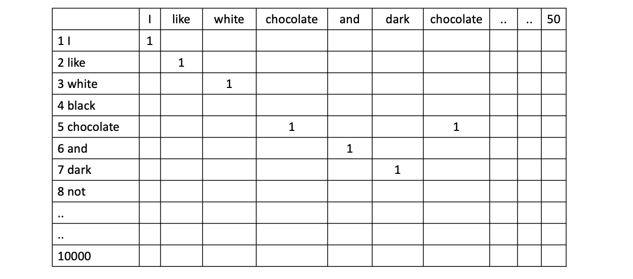
It will be a matrix of 50 columns X 10,000 rows = 500,000 elements.
That’s where a concept of embeddings come in. It is a matrix multiplication process which uses a smaller matrix to translate the big one hot matrix into a more manageable size to be passed to the RNNs
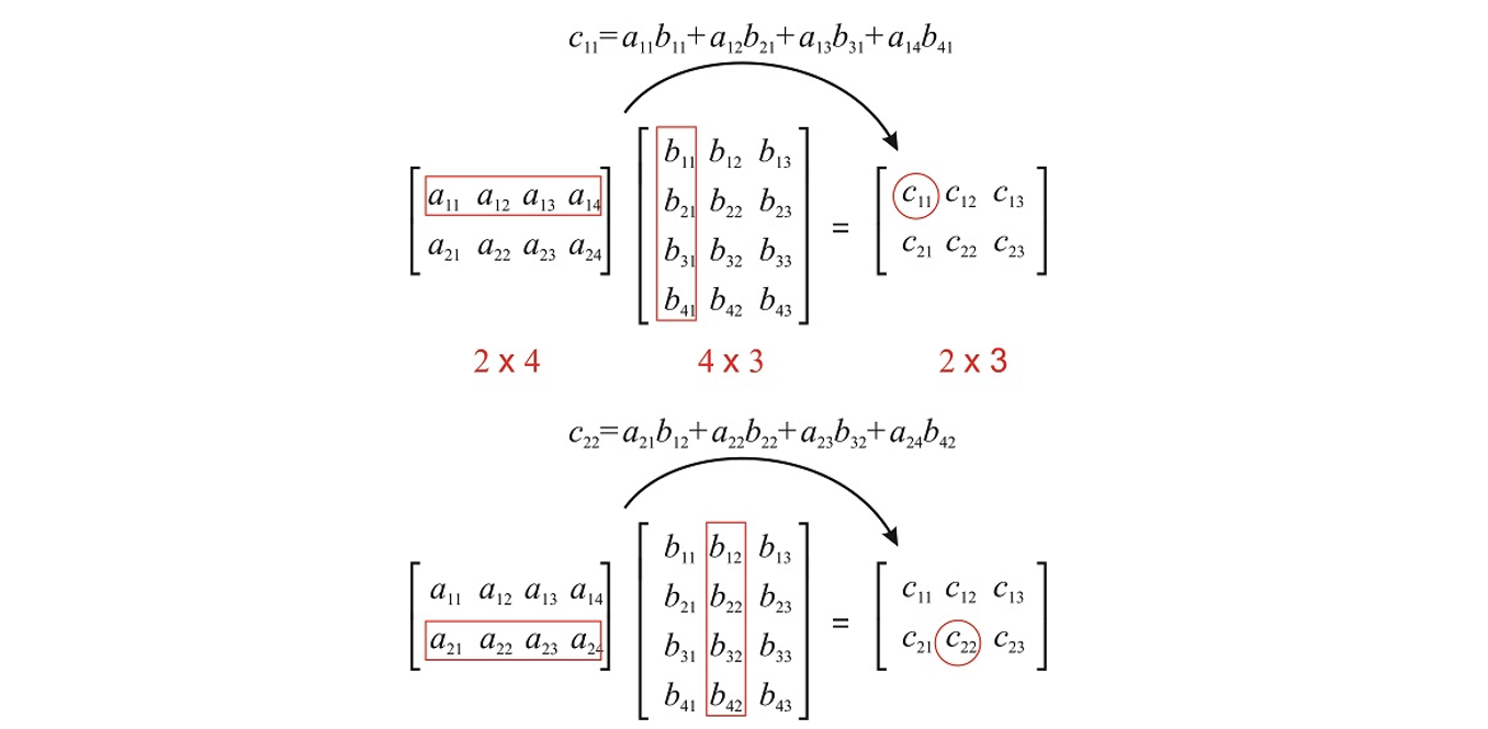
A small empty embeddings matrix is placed right before the input data goes to the RNN and when we train the model the embeddings are learned simultaneously. The embedding representation of the data generally means that it clubs words with similar meaning together after the learnings.

Recurrent Neural Networks
In a dense neural network while doing linear regression we pass all elements from 1 layer to the next, for example when we are addressing a linear regression problem like housing prices, the price of the house is based on sq ft, bedrooms, baths etc, but there is no actual relation that a high sq ft house will have more rooms. Even if it is, it can be learned. Language is much different, the order of words matter, their sequence needs to be preserved, as you will see below to couple of sections, all these RNN efforts are made to preserve significance of what words came before this word we are analyzing.
In a RNNs we send the information within a layer in order of the sentence sequence, and we process 1 layer sequence before we send the information to the next hidden layer.
Below we have an example of a sentence “I like to eat food”, the a1, a2, values gets passed within the first layer and for each neuron there are 2 inputs (a[t-1] and X[t]) and 2 outputs (a[t] and Y[t]).
This is an example of a one direction RNN, It can also be Bidirectional where the value from next neuron gets fed into previous neuron.
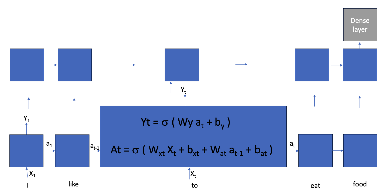
A simple representation of neuron used above can be represented as below where instead of sigmoid we are using tanh as activation function, generally in RNN we use tanh.

There is an argument that by the time the values are propagated left to right in a layer, the initial neuron affect becomes very minimal, this problem is called as Short Term Memory issue, so there are efforts to preserve some aspect of initial part of sequence by adding some more flows of data internally and using activation functions as gates.
LSTM – Long short-term memory, below is the traffic in a LSTM neuron. The inputs from X[t] passed through an activation function to act as a gate to control the amount of input which directly influences the outputs.

GRU – Gated Recurrent Unit, below is the traffic in a GRU neuron. It is a simpler version of LSTM
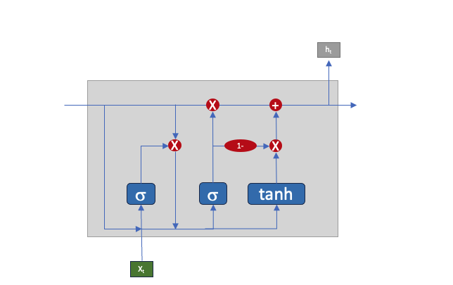
From a coding standpoint, the code is already there in the library and there is very minimal difference between them from a programming standpoint.
Simple RNN
model=tf.keras.models.Sequential([
  Input(shape=(SEQUENCE_LENGTH,)),
  Embedding(VOCAB_SIZE,EMBEDDING_DIM),
  SimpleRNN(32),
  Dense(1,activation='sigmoid'),
])
LSTM
model=tf.keras.models.Sequential([
  Input(shape=(SEQUENCE_LENGTH,)),
  Embedding(VOCAB_SIZE,EMBEDDING_DIM),
  Bidirectional(LSTM(64,return_sequences=True)),
  Bidirectional(LSTM(32)),
  Dense(64, activation='relu'),
  Dropout(0.5),
  Dense(1,activation='sigmoid'),
])
GRU
model=tf.keras.models.Sequential([
  Input(shape=(SEQUENCE_LENGTH,)),
  Embedding(VOCAB_SIZE,EMBEDDING_DIM),
  Bidirectional(GRU(64,return_sequences=True)),
  Bidirectional(GRU(32)),
  Dense(64, activation='relu'),
  Dropout(0.5),
  Dense(1,activation='sigmoid'),
])
Even though the diagrams above look very complex, the internals are actually very straightforward, you can see the actual implementation of a RNN and LSTM here
Simple RNN : https://github.com/keras-team/keras/blob/v2.12.0/keras/layers/rnn/simple_rnn.py
LSTM: https://github.com/keras-team/keras/blob/v2.12.0/keras/layers/rnn/lstm.py
You can also enhance LSTM to LSTM2 by overriding the core above in standard_lstm and call methods above.
Also the documentation is very extensive and the API usage with example are listed like
Simple RNN: https://www.tensorflow.org/api_docs/python/tf/keras/layers/SimpleRNN
Language translation
The training data for Language translation will contain a map of English to Spanish translation sets
Hello good morning how are you. -> Hola buenos dias como estas.
The translation model will contain 2 parts, an encoder and a decoder.
The idea here is that when we are translating, we are not coming up with entire spanish sentence in 1 go. We are generating one word at a time, while looking at 2 things
- The whole English sentence
- The part of Spanish sentence which we have already generated

So to train it we rewrite our input sentence like
Input [Hello good morning how are you] [Start ]. ->
Expected output [Start Hola]
Input [Hello good morning how are you] [Start Hola]. ->
Expected output [Start Hola buenos]
Input [Hello good morning how are you] [Start Hola buenos]. ->
Expected output [Start Hola buenos dias]
Input [Hello good morning how are you] [Start Hola buenos dias]. ->
Expected output [Start Hola buenos dias como]
Input [Hello good morning how are you] [Start Hola buenos dias como]. ->
Expected output [Start Hola buenos dias como estas]
Input [Hello good morning how are you] [Start Hola buenos dias como estas]. ->
Expected output [Start Hola buenos dias como estas END]
Now the Encoder will be a layer with the Inputs (containing English and partial spanish sentences)
And Decoder will be a layer with Expected output (also called shifted target)
Putting it together
### ENCODER
input = Input(shape=(ENGLISH_SEQUENCE_LENGTH,), dtype="int64", name="input_1")
x=Embedding(VOCAB_SIZE, EMBEDDING_DIM, )(input)
encoded_input=Bidirectional(GRU(NUM_UNITS), )(x)

### DECODER
shifted_target=Input(shape=(SPANISH_SEQUENCE_LENGTH,), dtype="int64", name="input_2")
x=Embedding(VOCAB_SIZE,EMBEDDING_DIM,)(shifted_target)
x = GRU(NUM_UNITS*2, return_sequences=True)(x, initial_state=encoded_input)

### OUTPUT
x = Dropout(0.5)(x)
target=Dense(VOCAB_SIZE,activation="softmax")(x)
seq2seq_gru=Model([input,shifted_target],target)

seq2seq_gru.compile(..)
seq2seq_gru.fit(..)
seq2seq_gru.predict(..)
BLEU score (Bi-Lingual Evaluation Understudy)
When we go through the fit process, we need to pass the loss function to optimize. Generic loss function does not serve a proper purpose for this.
For above translation
Hello good morning how are you. -> Hola buenos dias como estas.
If we say each word in predicted output has to present in expected output then the below table shows how it can go wrong

The BLEU score is a number between zero and one that measures the similarity of the machine-translated text to a set of high quality reference translations.
It keeps deleting the already matched word, to give a score of 0.2 in case of second usecase

Attention model
In 2016 Dzmitry Bahdanau published https://arxiv.org/pdf/1409.0473.pdf which is widely known as the Bahdanau Attention Model
He argued – In this paper, we conjecture that the use of a fixed-length vector is a bottleneck in improving the performance of this basic encoder–decoder architecture, and propose to extend this by allowing a model to automatically (soft-)search for parts of a source sentence that are relevant to predicting a target word, without having to form these parts as a hard segment explicitly
Where he creates a weightage for each word in the English sentence in determining the translated word. So in the below example “dias” output is heavily dependent on english word “morning” and somewhat dependent on some other words also.

To do this remember we were having output Y[t] going to the next layer in the model, we pass it through a dense layer to convert it to a single value for each word in the sequence. Then we normalize those across the sequence to have a sum of 1 across all of the words.
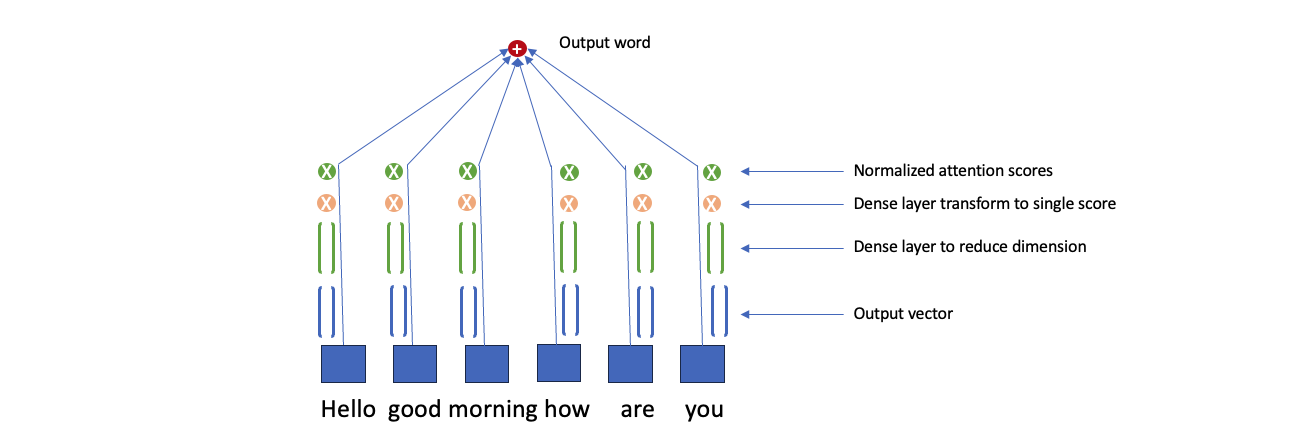
Picturizing the attention score in a heat map from his paper

Remember this attention model so far is creating a relation between the English sentence and the translated sentence.
In next post we will see how this got enhanced to the transformer model, and is now used to train GPT, BERT and other LLMs.
Cheers – Amit Tomar

