Quantum computing – maths

My next few posts will be about quantum computing, (not the Iran’s version where they portrayed a ZedBoard Zynq-7000 as a quantum processor).
We will code on IBM Qiskit libraries. This post will focus mainly on core concepts of linear algebra, complex numbers and mathematics for quantum computing.

Matrices

A matrix is a rectangular array of numbers, symbols, or expressions arranged in rows and columns. Matrices are widely used in linear algebra, computer science, physics, and engineering.

A matrix is typically written as:

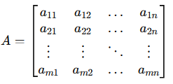
This matrix has m rows and n columns, it is called an m × n matrix.

Square Matrix: A matrix with equal rows and columns (m=n).

Row Matrix: A matrix with a single row (1×n).

Column Matrix: A matrix with a single column (m×1).

Identity Matrix: A square matrix where all diagonal elements are 1, and all off-diagonal elements are 0.

Zero Matrix: All elements are zero.

Diagonal Matrix: A square matrix where only the diagonal elements are nonzero.

Symmetric Matrix: A square matrix where A^T=A

Matrix Addition and Subtraction: If A and B have the same dimensions

Scalar Multiplication: Multiplying a matrix by a scalar k

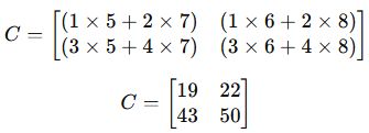
Matrix Multiplication: For two matrices A (m × n) and B (n × p) the resulting matrix will be C (m x p) where each element will be

Example

Transpose of a Matrix (A^T)

The transpose of a matrix A is obtained by flipping it along its main diagonal (switching rows and columns).

Complex Conjugate of a Matrix (A∗)

The complex conjugate of a matrix is obtained by replacing each element with its complex conjugate (changing i to −i).

Conjugate transpose of a Matrix

The conjugate transpose (also called the Hermitian adjoint, denoted as A† ) of a matrix A is obtained by:

• Taking the transpose of A (flipping it over its diagonal).
• Taking the complex conjugate of each entry.

Take the transpose

Take the complex conjugate of each element:

Unitary operator
A unitary operator is a linear operator UU on a Hilbert space that satisfies the condition:

U^† is the conjugate transpose (also called the Hermitian adjoint) of U.
I is the identity matrix.

is unitary if

Expanding this condition gives

This results in the conditions

Matrix Determinant

The determinant of a square matrix A (denoted as ∣A∣) is a scalar value that provides important information about the matrix.

For a 2×2 matrix:

the determinant is: |A| = ad − bc

For a 3×3 matrix:

the determinant is: |A| = a.(ei−fh) − b.(di−fg) + c.(dh−eg)

Expectation Value

Weighted sum of eigenvalues representing an observable in quantum mechanics.
In quantum mechanics, the expectation value of an observable A in a given quantum state ∣ψ⟩ is:

⟨A⟩=⟨ψ∣A∣ψ⟩

where:

• ∣ψ⟩ is a state vector,
• A is an operator (represented as a matrix),
• ⟨ψ∣A∣ψ⟩ is a quadratic form, essentially a weighted sum of eigenvalues.

Inner product

The inner product of matrices is typically defined as the sum of the element-wise product of two matrices of the same size. This is also known as the Frobenius inner product.

Example

Outer Product

The outer product of two matrices results in a larger matrix formed by multiplying elements of one with the elements of the other.

Example

Tensor Product

The tensor product is a fundamental operation in linear algebra that extends the concept of the outer product to higher-dimensional spaces. It is widely used in quantum mechanics, differential geometry, and machine learning.
Example

Eigenvalues and Eigenvectors

For a square matrix A of size n×n, an eigenvector v and an eigenvalue λ satisfy the equation: Av=λv

where:

• AA is an n×n matrix,
• v (the eigenvector) is a nonzero vector,
• λ (the eigenvalue) is a scalar.

This equation means that when A acts on v, it only scales it by λ, without changing its direction.

Finding Eigenvalues

Eigenvalues are found by solving the characteristic equation Determinant (A−λI) = 0

|A−λI|= 0

where:

• I is the identity matrix,
• |matrix| is the determinant of the matrix

Solving this equation gives the possible values of λ.

Finding Eigenvectors

Once the eigenvalues λ are found, eigenvectors are obtained by solving:

(A−λI).v = 0

This system finds nonzero solutions for v.

Expectation and Variance in Probability

Expectation (Expected Value, Mean)

The expectation E[X] of a random variable X represents the average or expected outcome if the experiment were repeated infinitely many times. It is a fundamental measure of the central tendency.
If X represents the outcome of rolling a fair 6-sided die, then:

Variance

Variance Var(X) measures how much a random variable deviates from its expected value. It quantifies the spread of the probability distribution.

From earlier, we know E[X]=3.5. Now, we calculate E[X2]:

Bra-Ket Notation (Dirac Notation)

Bra-ket notation, developed by Paul Dirac, is widely used in quantum mechanics to describe quantum states and their inner products in Hilbert space.

Kets ∣ψ⟩ – Column Vectors

A ket ∣ψ⟩ represents a quantum state, usually as a column vector.
For example, a two-state quantum system (like a qubit) might be:

where α,β are complex numbers.

Examples of standard basis kets in a 2D quantum system:

These correspond to quantum bits (qubits) in computational basis.

Bras ⟨ψ∣ – Row Vectors

A bra ⟨ψ∣ is the Hermitian conjugate (transpose + complex conjugate) of a ket.

For above mentioned Ket the corresponding bra is:

where α∗ and β∗ are the complex conjugates.

Inner Product (Bra-Ket ⟨ϕ∣ψ⟩ )

The inner product between two states ∣ϕ⟩ and ∣ψ⟩ is given by: ⟨ϕ∣ψ⟩ Which is a scalar output as defined in Inner products section above

Outer Product (∣ψ⟩⟨ϕ∣) – Matrix

The outer product of a ket and a bra forms a matrix: ∣ψ⟩ ⟨ϕ∣

Wavefunctions

In quantum mechanics, ψ represents a wavefunction or a state vector in Hilbert space. It is commonly used in matrix representations of quantum states, where a wavefunction ∣ψ⟩ is represented as a column vector.
For example, a quantum state in a two-level system (qubit) might be written as:

where α,β are complex numbers satisfying ∣α∣2 + ∣β∣ 2 = 1.

Polar Coordinate System

The polar coordinate system is a two-dimensional coordinate system where points are represented by their distance from a reference point and an angle from a reference direction (r,θ) where:

• r (radial coordinate) is the distance from the origin (pole).
• θ (angular coordinate) is the angle measured counterclockwise from the positive x-axis.

From Polar to Cartesian:

Given a point (r,θ), the Cartesian coordinates (x,y) are:
x = r . cos(θ)
y = r . sin(θ)

Bloch Sphere: Visualizing a Qubit in Quantum Computing

The Bloch sphere is a geometrical representation of a qubit, the fundamental unit of quantum information. It provides an intuitive way to visualize quantum states.

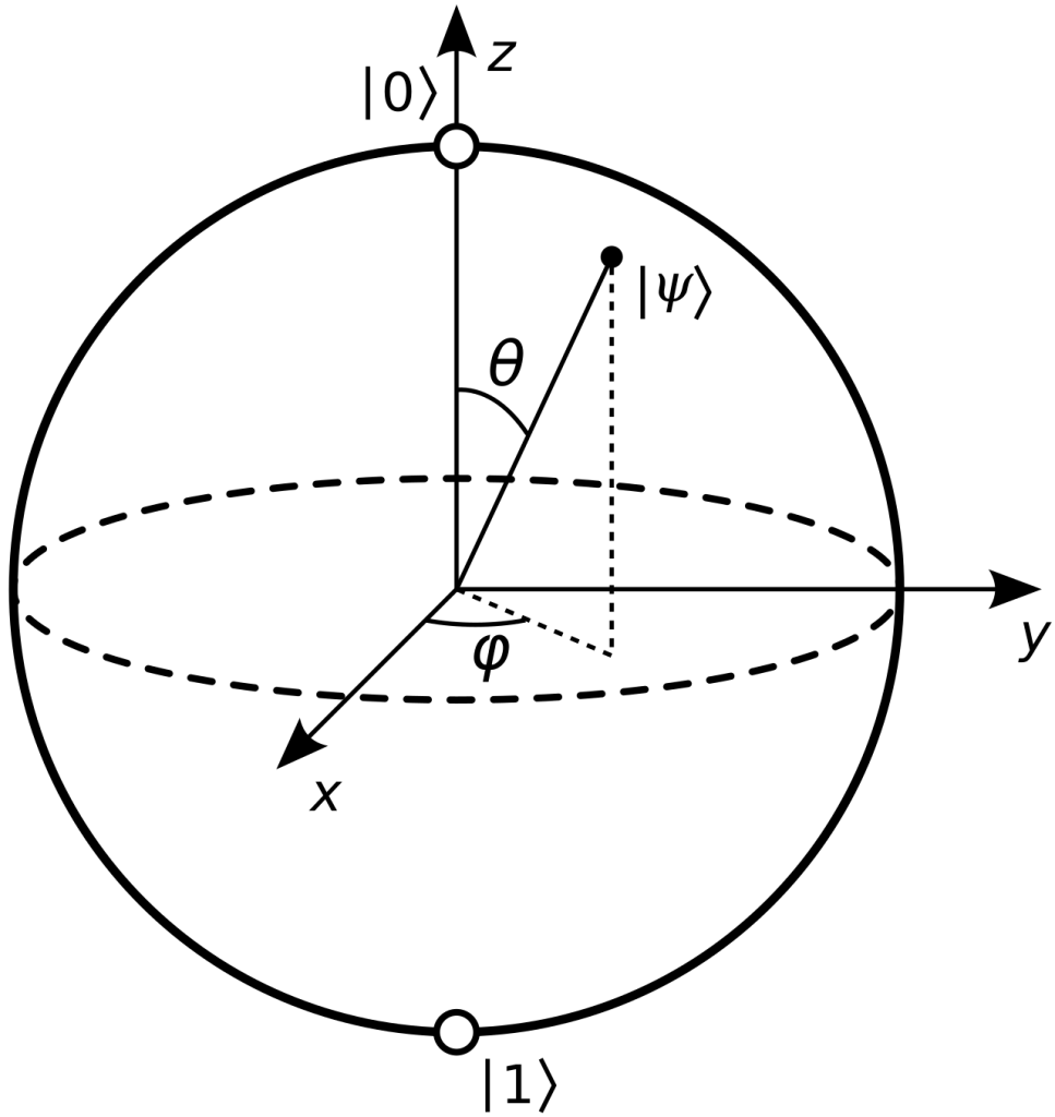
The quantum state of a single qubit is represented as:

where:

• ∣0⟩ and ∣1⟩ are the computational basis states.
• θ (polar angle) and ϕ (azimuthal angle) define the state on the Bloch sphere.
• The global phase does not affect the qubit state, so the sphere fully describes all possible single-qubit states.

Cartesian Coordinates on the Bloch Sphere

A qubit state can be expressed in terms of real coordinates:
x = sin θ cos ϕ
y = sin θ sin ϕ
z = cos θ

where:

• The z-axis represents classical 0 and 1 states.
• The x-y plane represents quantum superposition states.

Quantum Gates

Pauli-X Gate:

The Pauli-X gate, also called the quantum NOT gate, is a fundamental single-qubit gate in quantum computing. It flips the state of a qubit, just like the classical NOT operation.
The Pauli-X gate is represented by the 2×2 matrix:

It swaps the basis states:

Pauli-Y Gate:

The Pauli-Y gate is represented by the following 2×2 matrix:

So the Pauli-Y gate performs both a bit-flip and a phase flip

Pauli-Z Gate:

The Pauli-Z gate is represented by the following 2×2 matrix:

So, the Pauli-Z gate flips the phase of ∣1⟩, while leaving ∣0⟩ unchanged

Hadamard gate

The Hadamard gate is represented by the following 2×22×2 matrix

This creates superpositions where both ∣0⟩ and ∣1⟩ have equal amplitudes but with a relative phase in the case of ∣1⟩.

CODE

A Sample code for Pauli X gate, for Google colab

!pip install qiskit ipywidgets
!pip install qiskit-aer

import qiskit
import qiskit_aer
import numpy as np
from qiskit import QuantumCircuit, ClassicalRegister, QuantumRegister
from qiskit_aer import Aer
from qiskit.visualization import plot_bloch_multivector
from qiskit.visualization import plot_histogram
from math import pi, sqrt
from qiskit.quantum_info import Statevector

qr_x = QuantumRegister(1, "qr")
print ("qr_x:", qr_x)
print ("qr_x[0]:", qr_x[0])
sv = Statevector.from_int(0, dims=2)
print(sv)
plot_bloch_multivector(sv)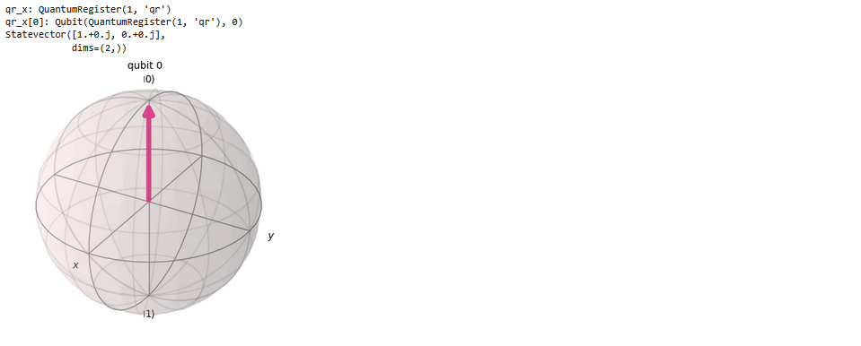

This shows the initial state as |0>

qc_x = QuantumCircuit(qr_x)
qc_x.x(qr_x[0])
qc_x.draw()

Here qr is initialized to 0, and after the X gate the value should be 1

backend = Aer.get_backend('statevector_simulator')
job = backend.run(qc_x)
result = job.result()
statevector = result.get_statevector()
# Print the statevector
print("\n Quantum State is: ", statevector)
plot_bloch_multivector(statevector)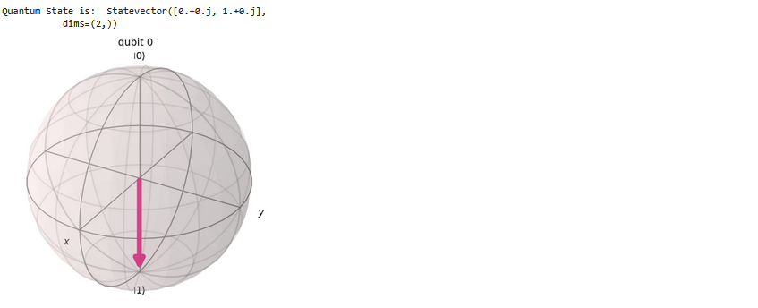

This is State 1 with matrix representation as [0,1]

backend = Aer.get_backend('unitary_simulator')
job = backend.run(qc_x)
result = job.result()
unitary = result.get_unitary()
# Print the unitary
print("\n Quantum State is: ", unitary)

This is the X operator matrix with value 0,1,1,0

cr_x = ClassicalRegister(1, "cr")
qr_x = QuantumRegister(1, "qr")
qc_x = QuantumCircuit(qr_x, cr_x)
qc_x.x(qr_x[0])
qc_x.measure(qr_x, cr_x)
qc_x.draw()

The Measurement operator will measure the value after Pauli X gate which should be 1

backend = Aer.get_backend('qasm_simulator')
job = backend.run(qc_x, shots=1024)
result = job.result()
counts = result.get_counts()
plot_histogram(counts)

This histogram shows 100% probability of 1 since we have applied Pauli X gate to single qubit.

Cheers!!

Amit Tomar