In the last post, I explained about matrix operations, the eigen vectors, the operator matrix, etc. We also went through the basic single qubit gates, like the Pauli X gate, Hadamard gate etc.
In this post we will cover multi Qubit Quantum gates and visualize the entanglement between states.
Quantum CNOT gate
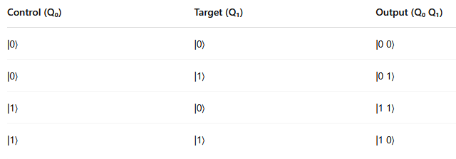
The quantum CNOT gate (Controlled-NOT gate) is a two-qubit quantum gate that flips the target qubit if and only if the control qubit is in state |1>. It’s one of the fundamental gates in quantum computing.
Let’s say we have two qubits:
- Control qubit: First qubit (Q₀)
- Target qubit: Second qubit (Q₁)
The CNOT gate behaves like this:
Basically:
- If the control qubit is |0⟩, do nothing.
- If the control qubit is |1⟩, flip the target qubit (|0⟩ ↔ |1⟩).
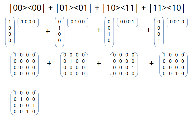
The operator matrix for CNOT gate is calculated to be a 4×4 matrix
The calculation for operator matrix goes as follows
Code for Quantum CNOT gate
!pip install qiskit ipywidgets
!pip install qiskit-aer
!pip install pylatexenc
Import the libraries
import qiskit
import numpy as np
from qiskit import QuantumCircuit, ClassicalRegister, QuantumRegister
from qiskit_aer import Aer
from qiskit import transpile
from qiskit.visualization import plot_state_city
from qiskit.visualization import plot_state_qsphere
from qiskit.visualization import plot_bloch_multivector
from qiskit.visualization import plot_histogram
from math import pi, sqrt
from qiskit.quantum_info import Statevector
Quantum CNOT/CX Gate
# CX-gate on |11> = |10> (|01> according to Qiskit ordering)
qc_cx = QuantumCircuit(2,name="qc")
qc_cx.x(0) # X Gate on 1st Qubit
qc_cx.x(1) # X Gate on 2nd Qubit
#Input to cx gate is 11 because of the X gates
qc_cx.cx(0,1) # CX Gate with 1st Qubit as Control and 2nd Qubit as Target
qc_cx.draw('mpl')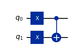
Density Matrix Plot for CNOT Gate
# To get the eigenvector we use the statevector simulator in the core of the circuit (without measurements)
simulator_state = Aer.get_backend('statevector_simulator')

# Execute the circuit
job_state = simulator_state.run(qc_cx)
result_state = job_state.result()

# Grab results from the job
#result_state = job_state.result()

# Returns counts
psi  = result_state.get_statevector(qc_cx)
print("\nQuantum state is:",psi)

# Plot a Density Matrix Plot
plot_state_city(psi)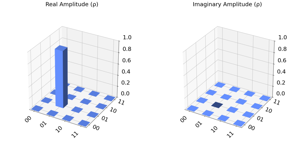
QSphere Plot for CX Gate
# Plot the QSphere
psi  = result_state.get_statevector(qc_cx)
plot_state_qsphere(psi)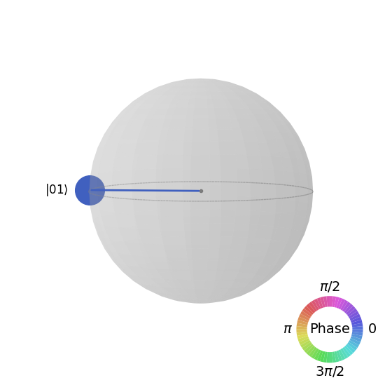
Unitary Operator for CNOT Gate
# Set the Aer simulator as Unitary for Unitary Operator
backend = Aer.get_backend('unitary_simulator')

# Execute the circuit
job = backend.run(qc_cx)
result_state = job.result()

result_state.get_unitary(qc_cx, decimals=3)
Output:
Operator([[0.+0.j, 0.+0.j, 0.+0.j, 1.+0.j],
[1.+0.j, 0.+0.j, 0.+0.j, 0.+0.j],
[0.+0.j, 1.+0.j, 0.+0.j, 0.+0.j],
[0.+0.j, 0.+0.j, 1.+0.j, 0.+0.j]],
input_dims=(2, 2), output_dims=(2, 2))Running CNOT Gate Circuit using QASM Simulator
# CNOT with Measurement
qc_cx = QuantumCircuit(2,2,name="qc")
qc_cx.x(0) # X Gate on 1st Qubit
qc_cx.x(1) # X Gate on 2nd Qubit
qc_cx.cx(0,1) # CX Gate with 1st Qubit as Control and 2nd Qubit as Target
qc_cx.measure([0,1],[0,1])
qc_cx.draw('mpl')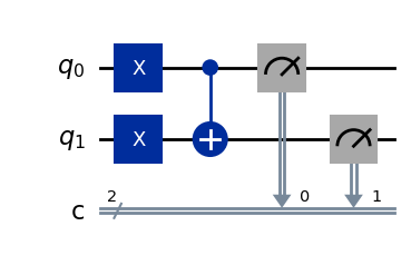
# Use Aer's qasm_simulator
backend = Aer.get_backend('qasm_simulator')

# Execute the circuit on the qasm simulator
job = backend.run(qc_cx, shots=1000)
# Grab results from the job
result = job.result()

# Returns counts
counts = result.get_counts(qc_cx)
print("\nTotal counts are:",counts)

# Plot a histogram
plot_histogram(counts)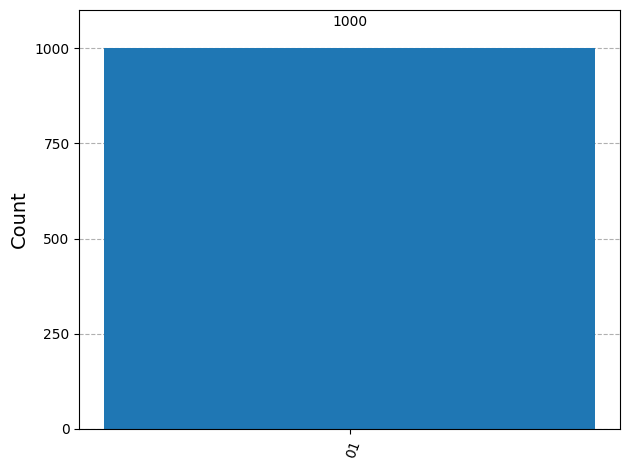
Quantum CH Gate
The Quantum CH gate, or Controlled-Hadamard gate, is a two-qubit gate where:
- The first qubit is the control.
- The second qubit is the target.
It applies a Hadamard gate to the target only if the control qubit is in state |1⟩.
The CNOT gate behaves like this:
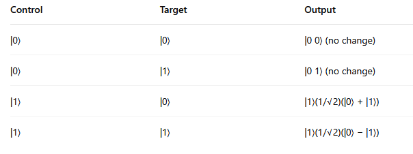
Basically:
- If control is |0⟩, nothing happens.
- If control is |1⟩, apply Hadamard to the target.
The operator matrix for CH gate is calculated to be a 4×4 matrix
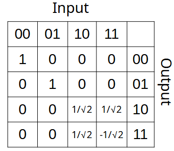
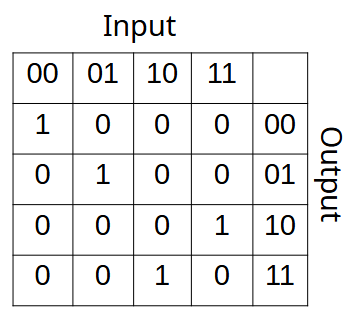
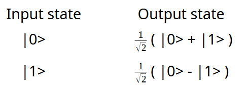
For a simple hadamard gate the Inputs and Outputs are as follows
Assume we pass |1> |1> to the Quantum CH gate. The Psi value, the row value calculations are shown below
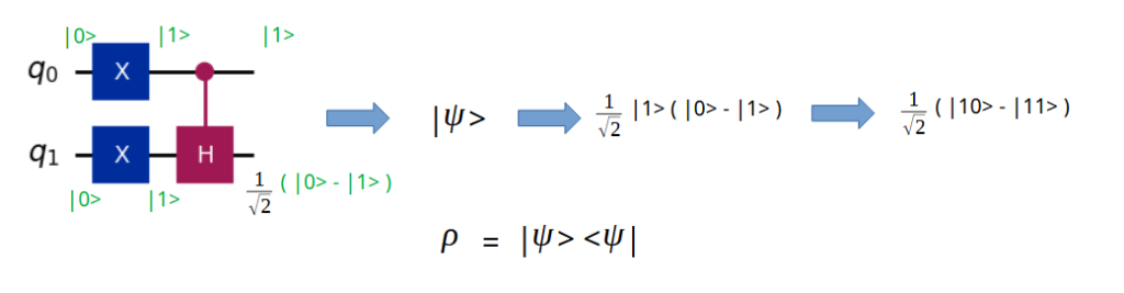
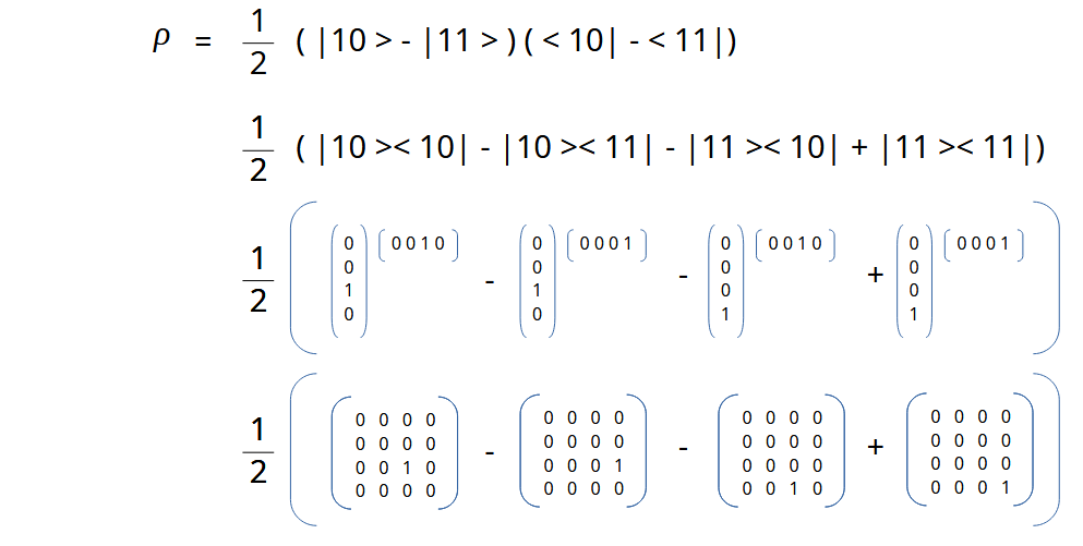
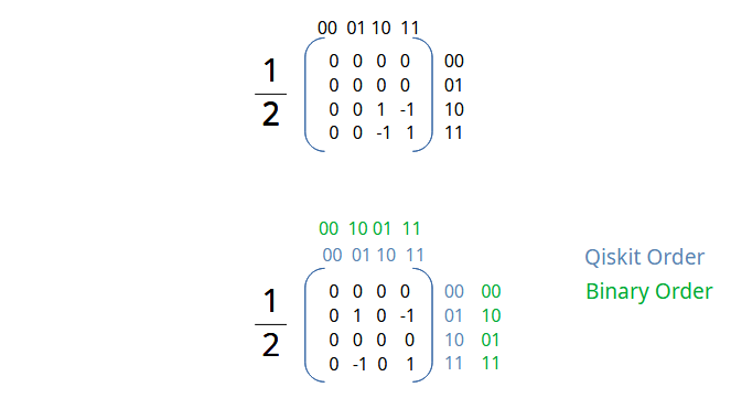
And expanding on the matrix notations as we did in our last post
Code for Quantum CH gate
# CH-gate on |11>
qc_ch = QuantumCircuit(2,name="qc")
qc_ch.x(0) # X Gate on 1st Qubit
qc_ch.x(1) # X Gate on 2nd Qubit
qc_ch.ch(0,1) # CH Gate with 1st Qubit as Control and 2nd Qubit as Target
qc_ch.draw('mpl')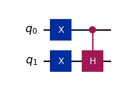
Density Plot for CH gate
# To get the eigenvector we use the statevector simulator in the core of the circuit (without measurements)
simulator_state = Aer.get_backend('statevector_simulator')

# Execute the circuit
# since CH gate is not preimplemented, we have to transpile to create one for us.
qc_ch_transpiled = transpile(qc_ch, simulator_state)
job_state = simulator_state.run(qc_ch_transpiled)

# Grab results from the job
result_state = job_state.result()

# Returns counts
psi  = result_state.get_statevector(qc_ch)
print("\nQuantum state is:",psi)

# Plot a Density Matrix Plot
plot_state_city(psi)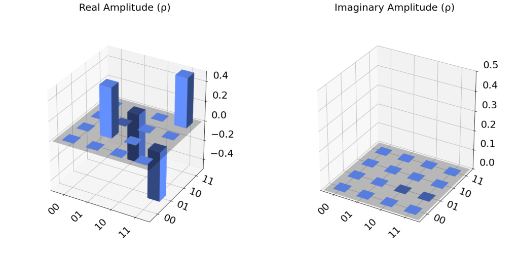
QSphere Plot for CH Gate
# Plot the QSphere
psi  = result_state.get_statevector(qc_ch)
plot_state_qsphere(psi)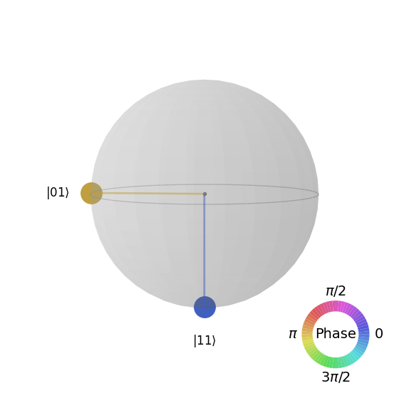
Unitary Operator for CH Gate
# Set the Aer simulator as Unitary for Unitary Operator
backend = Aer.get_backend('unitary_simulator')

# Execute the circuit
qc_ch_transpiled = transpile(qc_ch, backend)
ch_unitary = backend.run(qc_ch_transpiled)
ch_unitary.result().get_unitary(qc_ch, decimals=3)
Output:
Operator([[ 0. +0.j, -0. +0.j, 0. +0.j, 1. -0.j],
[ 0.707+0.j, 0. +0.j, 0.707+0.j, 0. +0.j],
[ 0. +0.j, 1. -0.j, 0. +0.j, -0. +0.j],
[-0.707+0.j, 0. +0.j, 0.707-0.j, 0. +0.j]],
input_dims=(2, 2), output_dims=(2, 2))Running CH Gate Circuit using QASM Simulator
# CH-gate on |11>
qc_ch = QuantumCircuit(2,2,name="qc")
qc_ch.x(0) # X Gate on 1st Qubit
qc_ch.x(1) # X Gate on 2nd Qubit
qc_ch.ch(0,1) # CH Gate with 1st Qubit as Control and 2nd Qubit as Target
qc_ch.measure([0,1],[0,1])
qc_ch.draw('mpl')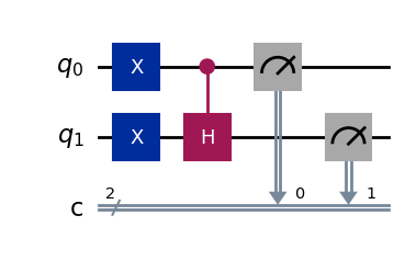
# Use Aer's qasm_simulator
backend = Aer.get_backend('qasm_simulator')

# Execute the circuit on the qasm simulator
qc_ch_transpiled = transpile(qc_ch, backend)
job = backend.run(qc_ch_transpiled, shots=1000)
# Grab results from the job
result = job.result()

# Returns counts
counts = result.get_counts(qc_ch)
print("\nTotal counts are:",counts)

# Plot a histogram
plot_histogram(counts)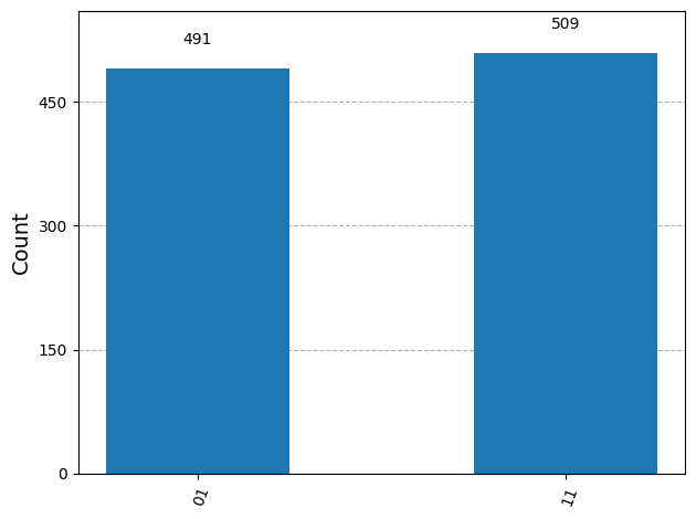
The Bell State
A Bell state is a special type of entangled quantum state involving two qubits. When two qubits are in a Bell state, measuring one qubit instantly determines the outcome of the other, even if they’re far apart. This is the heart of quantum entanglement.
There are 4 Bell states, all maximally entangled. The most common one is:

All four bell states are
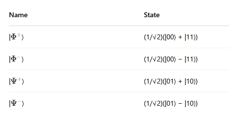
They form a complete orthonormal basis for two-qubit states and are central to:
- Quantum teleportation
- Superdense coding
- Quantum key distribution (QKD)
Assume we pass |0> |0> to the Bell gate. Notice now the Hadamard gate is controlling the CNOT gate
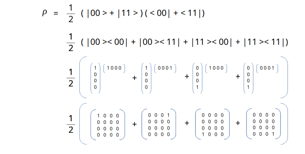
The Psi value, the row value calculations are shown below
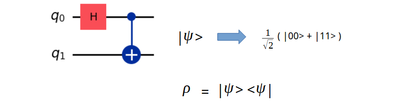
And expanding on the matrix notations as we did in our last posts
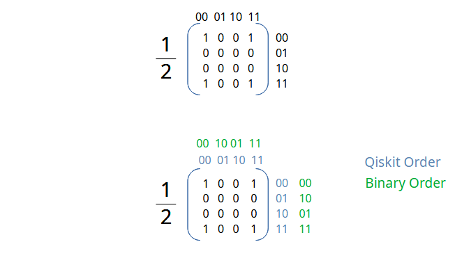
Code for The Bell state
# The Bell State
qc_bell = QuantumCircuit(2,2,name="qc")
qc_bell.h(0) # H Gate on 1st Qubit
qc_bell.cx(0,1) # CNOT with 1st as Control and 2nd as Target
qc_bell.draw(output='mpl')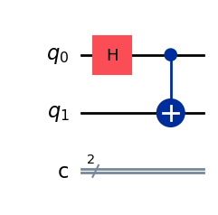
Density Matrix Plot for the Bell State
# To get the eigenvector you should use the statevector simulator in the core of the circuit (without measurements)
simulator_state = Aer.get_backend('statevector_simulator')

# Execute the circuit
job_state = simulator_state.run(qc_bell)
# Grab results from the job
result_state = job_state.result()

# Returns counts
psi  = result_state.get_statevector(qc_bell)
print("\nQuantum state is:",psi)

# Plot a Density Matrix Plot
plot_state_city(psi)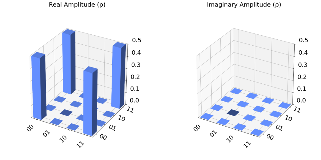
QSphere Plot for the Bell State
# Plot the QSphere
psi  = result_state.get_statevector(qc_bell)
plot_state_qsphere(psi)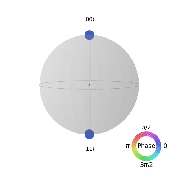
Unitary Operator for the Bell State
# Set the Aer simulator as Unitary for Unitary Operator
backend = Aer.get_backend('unitary_simulator')

# Execute the circuit
bell_unitary = backend.run(qc_bell)
bell_unitary.result().get_unitary(qc_bell, decimals=3)
Output:
Operator([[ 0.707+0.j, 0.707-0.j, 0. +0.j, 0. +0.j],
[ 0. +0.j, 0. +0.j, 0.707+0.j, -0.707+0.j],
[ 0. +0.j, 0. +0.j, 0.707+0.j, 0.707-0.j],
[ 0.707+0.j, -0.707+0.j, 0. +0.j, 0. +0.j]],
input_dims=(2, 2), output_dims=(2, 2))Running the Bell State Circuit on QASM Simulator
# The Bell State
qc_bell = QuantumCircuit(2,2,name="qc")
qc_bell.h(0) # H Gate on 1st Qubit
qc_bell.cx(0,1) # CNOT with 1st as Control and 2nd as Target
qc_bell.barrier()
qc_bell.measure([0,1],[0,1])
qc_bell.draw(output='mpl')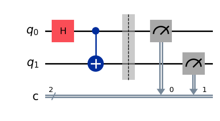
# Use Aer's qasm_simulator
backend = Aer.get_backend('qasm_simulator')

# Execute the circuit on the qasm simulator
job = backend.run(qc_bell, shots=1000)

# Grab results from the job
result = job.result()

# Returns counts
counts = result.get_counts(qc_bell)
print("\nTotal counts are:",counts)

# Plot a histogram
plot_histogram(counts)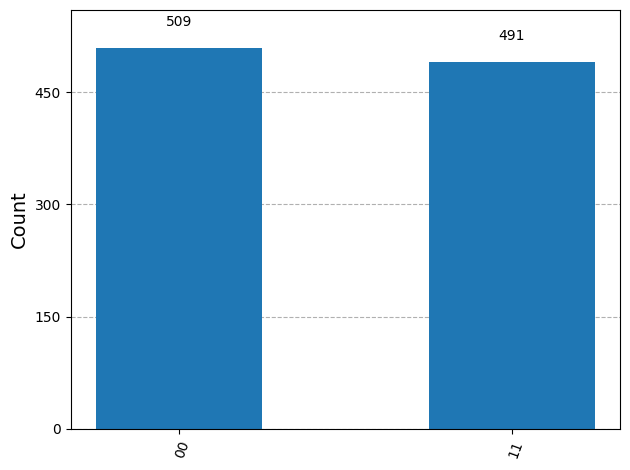
Cheers!!
Amit Tomar