We keep hearing about how AI has advanced because of deep learning. Lets see a comparison between a neural network vs a Linear regression model
Linear regression analysis is used to predict the value of a variable based on the value of another variable. We will use it to predict house prices, the dataset we are using is coming from Kaggle
Let’s jump into the code
First part is mostly data processing
import pandas as pd
import numpy as np
import matplotlib.pyplot as plt
import seaborn as sns
read the data from the local file
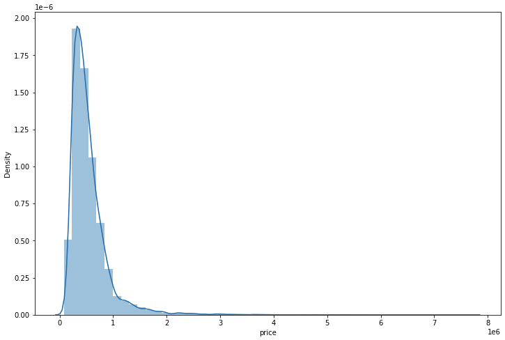
df = pd.read_csv('/content/sample_data/kc_house_data.csv')Lets plot a histogram for the price
plt.figure(figsize=(12,8))
sns.distplot(df['price'])
Drop the id and zipcode columns since it is not needed in training and look at the data
df = df.drop('id',axis=1)
df = df.drop('zipcode',axis=1)
We will translate the date to month and year to have a possibly meaningful pattern
df['date'] = pd.to_datetime(df['date'])
df['month'] = df['date'].apply(lambda date:date.month)
df['year'] = df['date'].apply(lambda date:date.year)
df = df.drop('date',axis=1)
We are now ready to extract training data as X and values as y
X = df.drop('price',axis=1)
y = df['price']
Split the data 70 / 30 into train and test sets
from sklearn.model_selection import train_test_split
X_train, X_test, y_train, y_test = train_test_split(X,y,test_size=0.3,random_state=50)
Scale the data to values between 0 and 1 to reduce impact of large value columns
from sklearn.preprocessing import MinMaxScaler
scaler = MinMaxScaler()
X_train= scaler.fit_transform(X_train)
X_test = scaler.transform(X_test)
Building out the tensor models
from tensorflow.keras.models import Sequential
from tensorflow.keras.layers import Dense, Activation
from tensorflow.keras.optimizers import Adam

model = Sequential()

model.add(Dense(19,activation='relu'))
model.add(Dense(19,activation='relu'))
model.add(Dense(19,activation='relu'))
model.add(Dense(19,activation='relu'))
model.add(Dense(1))

model.compile(optimizer='adam',loss='mse')
Fit Fit already, ok lets use 400 epochs, we could have used callbacks, but this is just an example.
model.fit(x=X_train,y=y_train.values,
           validation_data=(X_test,y_test.values),
           batch_size=128,epochs=400)
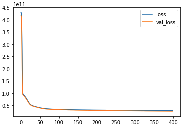
The training logs to show the reducing error
Epoch 1/400
119/119 [==============================] - 2s 5ms/step - loss: 430236008448.0000 - val_loss: 418893430784.0000
Epoch 2/400
119/119 [==============================] - 0s 3ms/step - loss: 428638240768.0000 - val_loss: 413131243520.0000
Epoch 3/400
119/119 [==============================] - 0s 4ms/step - loss: 404477181952.0000 - val_loss: 357757026304.0000
Epoch 4/400
119/119 [==============================] - 0s 3ms/step - loss: 293354504192.0000 - val_loss: 194056830976.0000
Epoch 5/400
119/119 [==============================] - 0s 4ms/step - loss: 135950188544.0000 - val_loss: 97320124416.0000
..........
..........
Epoch 395/400
119/119 [==============================] - 1s 5ms/step - loss: 28670298112.0000 - val_loss: 26218856448.0000
Epoch 396/400
119/119 [==============================] - 1s 5ms/step - loss: 28637747200.0000 - val_loss: 26361298944.0000
Epoch 397/400
119/119 [==============================] - 1s 5ms/step - loss: 28653010944.0000 - val_loss: 26207547392.0000
Epoch 398/400
119/119 [==============================] - 1s 5ms/step - loss: 28645316608.0000 - val_loss: 26239582208.0000
Epoch 399/400
119/119 [==============================] - 1s 5ms/step - loss: 28662179840.0000 - val_loss: 26785748992.0000
Epoch 400/400
119/119 [==============================] - 1s 5ms/step - loss: 28646553600.0000 - val_loss: 26193301504.0000
<keras.callbacks.History at 0x7f7aa5e1e6a0>
Now lets plot the error rate decrease to show how the training went.
losses = pd.DataFrame(model.history.history) losses.plot()
Lets predict on test data
deep_predictions = model.predict(X_test)Now we move to Linear regression modelfrom sklearn.linear_model import LinearRegression
lm = LinearRegression() lm.fit(X_train,y_train)This is prediction on LM modellm_predictions = lm.predict(X_test)
Time to compare the 2 predictions
from sklearn.metrics import mean_squared_error,mean_absolute_errorWe see the mean absloute error (average of predicted vs real values) is less for NN/deep model
mean_absolute_error(y_test,deep_predictions)
100662.43128616898

mean_absolute_error(y_test,lm_predictions)
123998.5721289351
Also the RMSE (root mean squared) value of error are smaller for NN modelnp.sqrt(mean_squared_error(y_test,deep_predictions)) 161843.4469408165 np.sqrt(mean_squared_error(y_test,lm_predictions)) 201080.55278529547
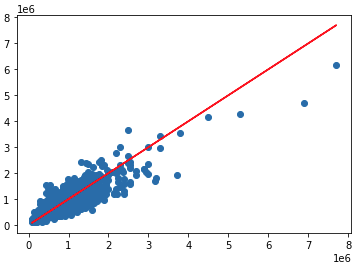
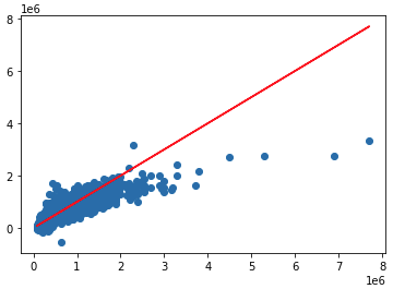
Lets plot the predicted vs real values
Deep model vs real
plt.scatter(y_test,deep_predictions)
plt.plot(y_test,y_test,'r')
Linear regression vs real
plt.scatter(y_test,lm_predictions)
plt.plot(y_test,y_test,'r')
We see the LM predictions are deviating from the real price line by quite a bit.
Let’s compare prediction for a single house
House 1
Here real price was 221K, NN predicted 288K and LM predicted 251K so LM wins
df.iloc[0]
price            221900.0000
bedrooms              3.0000
bathrooms             1.0000
sqft_living        1180.0000
sqft_lot           5650.0000

single_house = df.drop('price',axis=1).iloc[0]
single_house
bedrooms            3.0000
bathrooms           1.0000
sqft_living      1180.0000
sqft_lot         5650.0000

single_house = scaler.transform(single_house.values.reshape(-1, 19))

model.predict(single_house)
288092.03

lm.predict(single_house)
251823.61285049
House 2
Here real price was 662K, NN predicted 686K and LM predicted 845K so NN wins
df.iloc[10]
price            662500.0000
bedrooms              3.0000
bathrooms             2.5000
sqft_living        3560.0000
sqft_lot           9796.0000

single_house = df.drop('price',axis=1).iloc[10]

single_house
bedrooms            3.0000
bathrooms           2.5000
sqft_living      3560.0000
sqft_lot         9796.0000

single_house = scaler.transform(single_house.values.reshape(-1, 19))

model.predict(single_house)
686754.56

lm.predict(single_house)
845134.80613535
Well we do see the NN model predictions are much closer to the actual values in the test data.
I will write up similar example on Logistic regression and unsupervised learning to compare these again later on.
Cheers – Amit Tomar


