K-Means vs Neural network

When we think about a classification use-case the first thought which comes to mind is K-Means algorithim.

It tries to divide the dataset into K clusters. The basic steps on how it works is

Assign all points randomly to K clusters
Calculate the centeroid of each cluster
Then all points are assigned to their closest centeroid
Then for those points we re-calculate the centeroid
Keep repeating 3-4 till the data points are no longer assigned to a different cluster

This is a perfect textbook case of unsupervised learning

What we will do today is compare this unsupervised learning to a supervised learning with Neural Network

We will use the dataset as a generated blobs using scikit library which generates some data points in clusters and gives us the clusters too

Here is the code

Imports

import seaborn as sns 
import matplotlib.pyplot as plt 
%matplotlib inline

Make 2 blobs and display the in a chart

from sklearn.datasets import make_blobs

data = make_blobs(n_samples=1000, n_features=2,
                           centers=2, cluster_std=1.8,random_state=50)

plt.scatter(data[0][:,0],data[0][:,1],c=data[1],cmap='rainbow')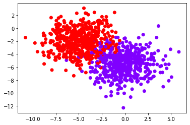

Use K-Means to distribute same data in 2 clusters

from sklearn.cluster import KMeans

kmeans = KMeans(n_clusters=2)

kmeans.fit(data[0])

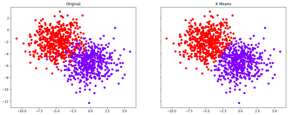
Lets see how the K-Means distributed the above data into clusters

f, (ax1, ax2) = plt.subplots(1, 2, sharey=True,figsize=(16,6))
ax1.set_title('K Means')
ax1.scatter(data[0][:,0],data[0][:,1],c=kmeans.labels_,cmap='rainbow')
ax2.set_title("Original")
ax2.scatter(data[0][:,0],data[0][:,1],c=data[1],cmap='rainbow'))

See in the original the blobs had some overlap, but K-Means made a clean cut

Lets use the same input, but use it as supervised learning in Neural networks

from tensorflow.keras.models import Sequential
from tensorflow.keras.layers import Dense, Activation
from tensorflow.keras.optimizers import Adam

# Setup the model
model = Sequential()
model.add(Dense(units=20, activation='relu'))
model.add(Dense(units=20, activation='relu'))
model.add(Dense(units=1, activation='sigmoid'))
model.compile(optimizer='adam',
              loss='binary_crossentropy')

Now fit the data in the model

import pandas as pd
X = pd.DataFrame(data[0])
y = pd.DataFrame(data[1])
from sklearn.model_selection import train_test_split

X_train, X_test, y_train, y_test = train_test_split(X, y,
                                   test_size=0.3, random_state=101)

# Train the model
history = model.fit(x=X_train, y=y_train,
                    epochs=200,
                    batch_size=256,
                    shuffle=True,
                    validation_data=(X_test, y_test),
                    verbose=1)

The training output

Epoch 1/200
3/3 [==============================] - 4s 272ms/step - loss: 0.6569 - val_loss: 0.5972
Epoch 2/200
3/3 [==============================] - 0s 33ms/step - loss: 0.5854 - val_loss: 0.5270
Epoch 3/200
3/3 [==============================] - 0s 42ms/step - loss: 0.5221 - val_loss: 0.4656
Epoch 4/200
3/3 [==============================] - 0s 62ms/step - loss: 0.4649 - val_loss: 0.4128
Epoch 5/200
3/3 [==============================] - 0s 45ms/step - loss: 0.4167 - val_loss: 0.3677
...............
Epoch 195/200
3/3 [==============================] - 0s 24ms/step - loss: 0.1058 - val_loss: 0.1077
Epoch 196/200
3/3 [==============================] - 0s 34ms/step - loss: 0.1059 - val_loss: 0.1078
Epoch 197/200
3/3 [==============================] - 0s 23ms/step - loss: 0.1058 - val_loss: 0.1078
Epoch 198/200
3/3 [==============================] - 0s 33ms/step - loss: 0.1058 - val_loss: 0.1077
Epoch 199/200
3/3 [==============================] - 0s 37ms/step - loss: 0.1058 - val_loss: 0.1078
Epoch 200/200
3/3 [==============================] - 0s 37ms/step - loss: 0.1057 - val_loss: 0.1077

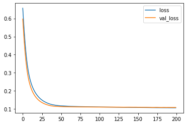
Plot the loss graph

Predict the classification, translate to 0/1 as 2 groups

import numpy as np

deep_predictions  = ((model.predict(X_test) > 0.5)).astype("int32").flatten()

Lets see how the classifications look compared to K-Means

f, (ax1, ax2, ax3) = plt.subplots(1, 3, sharey=True,figsize=(21,6))
ax1.set_title("Original")
ax1.scatter(data[0][:,0],data[0][:,1],c=data[1],cmap='rainbow')
ax2.set_title('K Means')
ax2.scatter(data[0][:,0],data[0][:,1],c=kmeans.labels_,cmap='rainbow')
X_test_arr = np.array(X_test)
ax3.set_title('Deep')
ax3.scatter(X_test_arr[:,0],X_test_arr[:,1],c=deep_predictions,cmap='rainbow')

The last plot is for the 30% test data only.

Looks good to me, both K-Means and Neural network performed well in this case.

Cheers – Amit Tomar

K-Means vs Neural network

Related Posts