In machine learning we try to understand the data, we train a model using the data and results we already have, and ask it to take a guess about the results for data where the results are not available, which we expect it to positively predict to a good deal of accuracy. If we see a person or an animal in the picture we are able to classify it correctly with a good confidence. We ask the machine to do a similar classification based on the data we can provide it.
In my last post, we talked about how to predict the house prices based on area, neighborhood and couple of other attributes. We built out some code to teach the model how to derive a price based on these attributes and then gave it some more data and asked it to predict the prices. The predictions were correct to a certain extent, and one could argue “we did not know every single value which can impact the price so obviously there is a margin of error”, well yes there is seller’s mood, agent’s skill, road conditions, paint color everything matters.
So why not give the machine some data which we can predict 100% of the time based on 5 attributes. I generated some data based on 5 random numbers A B C D E. The resulting column price is calculated as
PRICE = 100 X A + 200 X B^2 + 300 X C^3 + 400 X D^4 + 500 X E^5
We give some values of A B C D E and price data to the model training and see if it can figure out the formula.
The imports
import pandas as p
import numpy as np
import matplotlib.pyplot as plt
import seaborn as snsd
read and display the file contents
df = pd.read_csv('/content/sample_data/random.csv')
df.head()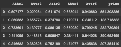
Separate out the target variable
X = df.drop('price',axis=1)
y = df['price']
Split the data into training and test set
from sklearn.model_selection import train_test_split
X_train, X_test, y_train, y_test = train_test_split(X,y,test_size=0.3,random_state=101)
Build the model, I tried with smaller models and results were not very accurate
from tensorflow.keras.models import Sequential
from tensorflow.keras.layers import Dense, Activation
from tensorflow.keras.optimizers import Adam
model = Sequential()

model.add(Dense(20,activation='relu'))
model.add(Dense(20,activation='relu'))
model.add(Dense(20,activation='relu'))
model.add(Dense(20,activation='relu'))
model.add(Dense(1))

model.compile(optimizer='adam',loss='mse')
Train the model
model.fit(x=X_train,y=y_train.values,
          validation_data=(X_test,y_test.values),
          batch_size=128,epochs=400)

Epoch 1/400
55/55 [==============================] - 3s 16ms/step - loss: 160081.3594 - val_loss: 158808.9062
Epoch 2/400
55/55 [==============================] - 0s 9ms/step - loss: 149142.0312 - val_loss: 129467.4453
Epoch 3/400
55/55 [==============================] - 0s 6ms/step - loss: 78614.5703 - val_loss: 26477.0391
Epoch 4/400
55/55 [==============================] - 0s 4ms/step - loss: 20834.4121 - val_loss: 20642.1406
Epoch 5/400
55/55 [==============================] - 0s 4ms/step - loss: 19614.5625 - val_loss: 19911.6914
......................
......................
Epoch 395/400
55/55 [==============================] - 0s 6ms/step - loss: 32.4420 - val_loss: 32.9228
Epoch 396/400
55/55 [==============================] - 0s 5ms/step - loss: 33.2386 - val_loss: 33.4047
Epoch 397/400
55/55 [==============================] - 0s 5ms/step - loss: 32.7264 - val_loss: 36.3450
Epoch 398/400
55/55 [==============================] - 0s 4ms/step - loss: 33.1888 - val_loss: 39.2235
Epoch 399/400
55/55 [==============================] - 0s 4ms/step - loss: 33.8868 - val_loss: 34.0010
Epoch 400/400
55/55 [==============================] - 0s 4ms/step - loss: 34.4255 - val_loss: 32.9567
<keras.callbacks.History at 0x7f433542d430>
Let’s plot the losses
losses = pd.DataFrame(model.history.history)
losses.plot()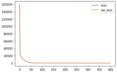
The predictions
deep_predictions = model.predict(X_test)Now lets use the Linear regression model for same thing
from sklearn.linear_model import LinearRegression
lm = LinearRegression()
lm.fit(X_train,y_train)

# Linear model predictions
lm_predictions = lm.predict(X_test)
Now lets look at the errors
The Mean absolute error from the neural model looks better than the one from from linear regression model
from sklearn.metrics import mean_squared_error,mean_absolute_error

mean_absolute_error(y_test,deep_predictions)
4.533919159991981

mean_absolute_error(y_test,lm_predictions)
77.65957671594275
The RMSE value also from neural model looks better
np.sqrt(mean_squared_error(y_test,deep_predictions))
5.740796915674413

np.sqrt(mean_squared_error(y_test,lm_predictions))
96.82128372203124
Scatter plot for Neural network predictions
# Our prediction
plt.scatter(y_test,deep_predictions)

# Perfect predictions
plt.plot(y_test,y_test,'r')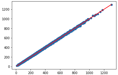
And the plot for predictions from linear regression model
# Our prediction
plt.scatter(y_test,lm_predictions)
# Perfect predictions
plt.plot(y_test,y_test,'r')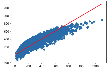
The neural network model was able to identify the correct formula we used and was able to predict the remaining values with very high level of accuracy.
Not bad, eh?
Cheers – Amit Tomar

