GAN: Diffusion Model

A generative adversarial network (GAN) is a class of machine learning frameworks and a prominent framework for approaching generative AI.
The core idea of a GAN is based on the “indirect” training through the discriminator, another neural network that can tell how “realistic” the input seems, which itself is also being updated dynamically. This means that the generator is not trained to minimize the distance to a specific image, but rather to fool the discriminator. This enables the model to learn in an unsupervised manner.

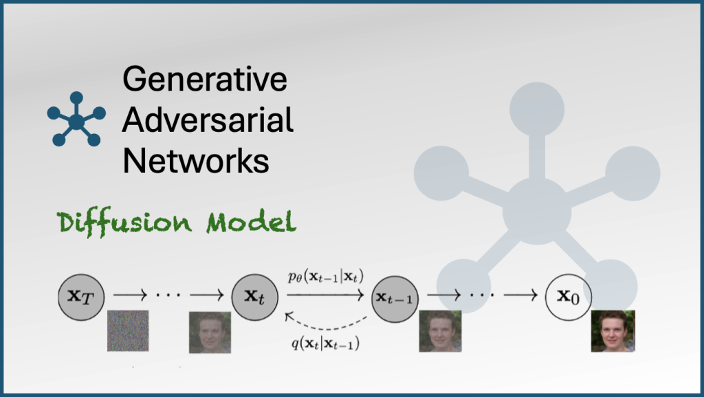
We are going to look at a Diffusion model which utilizes the transformer model. The model we are going to look at is Denoising Diffusion Probabilistic Models

The training for this model is done using images to which we add noise progressively, and train the model to remove the noise and generate the given image.

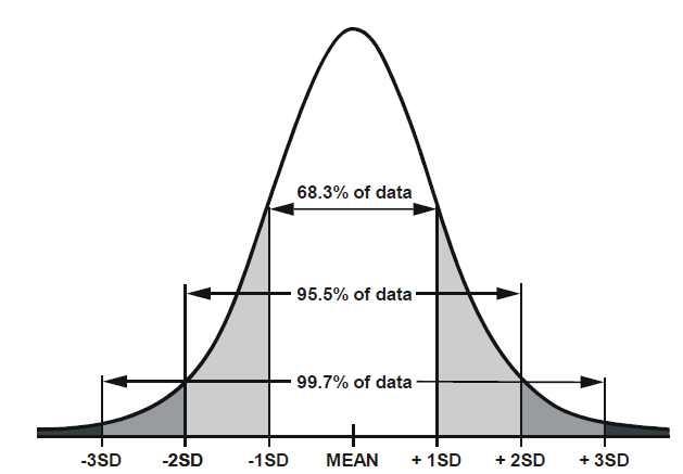
The noise is generated using values picked from normal distribution where the values closer to the mean have a higher probability to be picked.

To Add noise to the image, if we go from Zero to T steps adding more noise at each step, then q(X[t] | X[t-1]) is the probablity to get the image X[t] given the image X[t-1]

q is defined as a normal distribution which depends on X[t-1]. The Mean is the middle portion of the above equation and variance is beta[t]. And this is a normal distribution, so if beta[t] is zero, the X[t] is very highly dependent on X[t-1], but if beta[t] goes closer to 1, then X[t-1] has very little influence on the value of X[t].

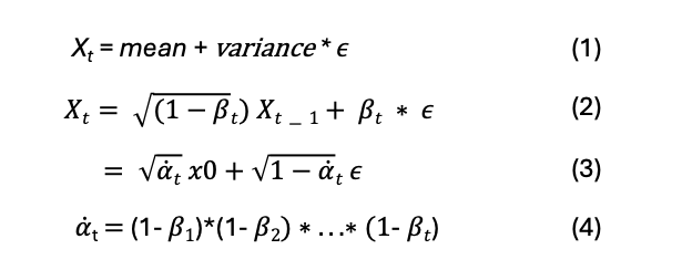
So X[t] is derived from mean and variance and a small value (e) which is derived from normal distribution and is close to zero.
The mean as per above equation is the square root of (1 – beta[t]).
If we want to derive X[t] all the way from X[0] then we can substitute (1 – beta[t]) with alpha[t] where alpha[t] will be a product of all the (1 – beta[t]) where t ranges from 1 to t

Now to obtain P

It is a inverse operation of Q, as per bayes theorem.

So now we know the values of all variables, since we are the ones generating the noise for the training, so alpha, beta, and images are all known. The only part unknown is the value of epsilon theta (X[t], t) which is needed to receate X[t-1]. So we can train the model to predict epsilon theta, which in other words is predicting the noise in the image, so we can subtract the noise from X[t] and produce X[t-1]

Training Algorithm

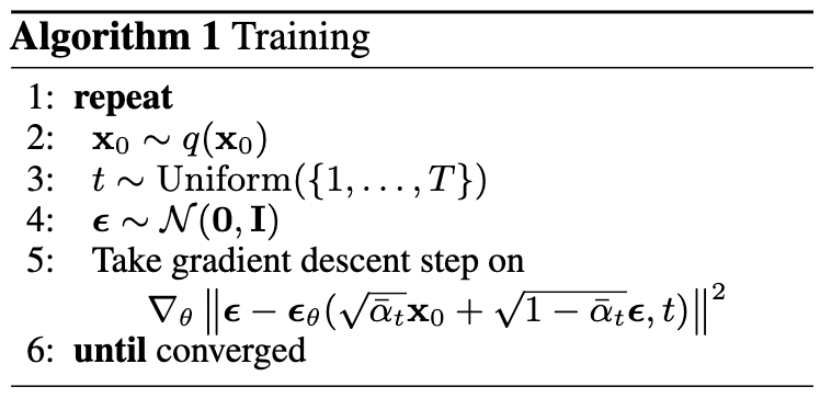
We pick the person’s picture from training data as x0
We pick a value of t from 1 to T
then we pick epsilon from 0 to 1
In gradient decent step, the model will predict epsilon theta, rest all the parameters in the equation are know, epsilon (the noise), x[0], alpha and t are all known. The vaule in parentheses is actually the noisy image which we generate based on epsilon and t, So our loss is the difference between epsilon and epsilon theta.

Sampling Algorithm

starting from a pre-generated random noise
Using our model which can now predict the noise which needs to be extracted out to build a less noisier image, we use the model to predict epsilon theta
When we plug this value in equation 4 above we get less noisy image X[t-1] for the given noisy image X[t], and we repeat the process T times to get a clear image from noise.

Code

The code for Denoising Diffusion Probabilistic Models is made available by authors at https://github.com/hojonathanho/diffusion

The model will take 2 inputs as shown in Step 5 of Training Algorithm, 1 – the noisy image, 2 – the value of t (we will use positional embedding for this as we will be using transformer model).
The model will them output the noise which is also a image which needs to be subtracted from the original image.
We will use the Unet model to down sample and up-sample the image to obtain the noise as output from the image.

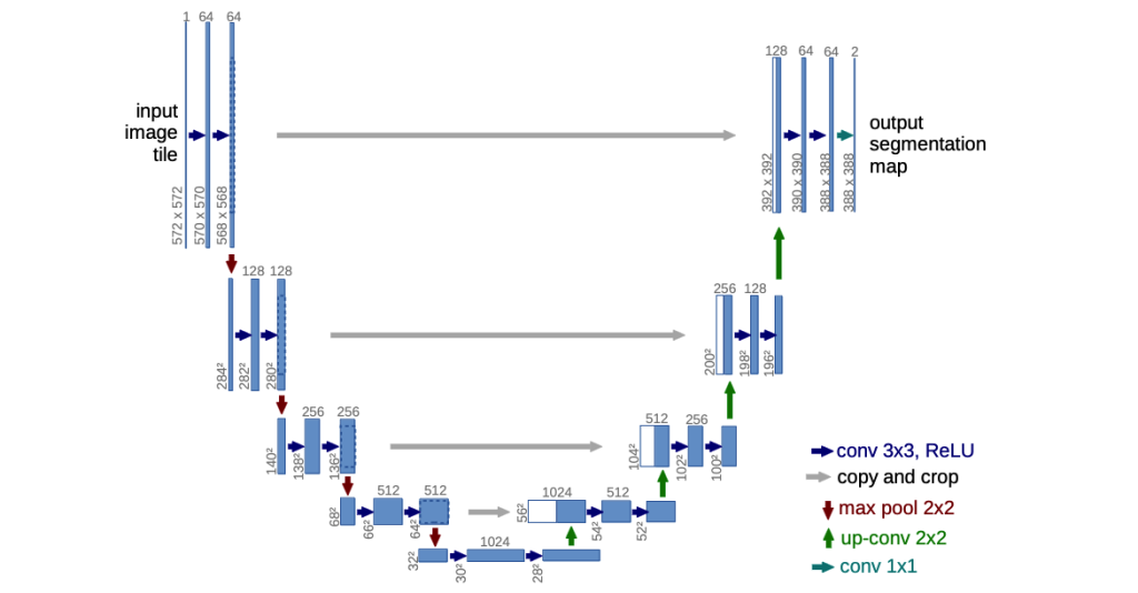
Code here https://github.com/hojonathanho/diffusion/blob/master/diffusion_tf/models/unet.py

Model (inputImage, timestep) {

    positionalEmbeddings (timestep) // the output of this goes into all the resnet blocks below along with input image
    Conv2d block

    # Downsample loop for channels 32, 64, 128, 256
    resnet block
    add resnet output inputforUpSampling to connect the gray lines to upsampling
    maxpooling2d (the downward red arrow)

    #Bottleneck layer - the bottom row in unet model
    Add 2 resnet blocks

    # UpSample loop in reverse channel 256, 128, 64, 32
    Input from previous input + inputforUpSampling.pop
    resnet block
    Conv2DTranspose for Upsampling (The green upward arrow)

    2 resnet blocks
    return output
}

Getting the positional embedding https://github.com/hojonathanho/diffusion/blob/master/diffusion_tf/nn.py
Method get_timestep_embedding
This process is very similar to building positional embedding in a transformer model. This step preserves the relevance of sequence of input data. In a NLP problem this creates a vector to keep the information of all the input text so that we do not lose relevance of sequence of words in the input.

In the model we get the positional embedding based on input t (aka timestep) and pass it through a Dens layer with Gelu activation GAUSSIAN ERROR LINEAR UNITS (GELUS)

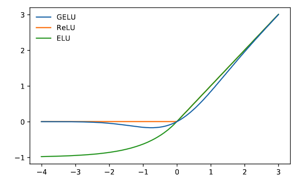
This is a probablity based activation layer, if a value is less then zero then we will have a y value which has a higher probablity (not definetly) of being non zero. Meaning for a x = -1 we may have y = 0 or y = -0.01 or y = -0.02, but having a non zero will be higher probablity compare to x = -3.

Resnet block https://github.com/hojonathanho/diffusion/blob/master/diffusion_tf/models/unet.py Method: resnet_block

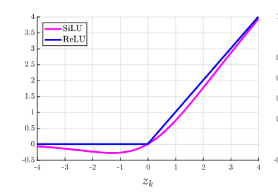
Has 2 conv layers with a residual connection joining the second conv layer after being processed by another conv layer. It uses group normalization https://arxiv.org/pdf/1803.08494 rather than batch normalization. It uses SiLU activation https://arxiv.org/pdf/1702.03118 for its conv layer.

Attention model

The Attention model was originally documented by Dzmitry Bahdanau in the paper Neural Machine Translation

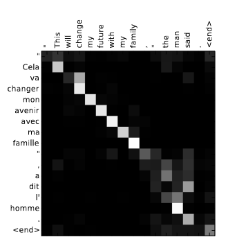
Since this was initially used for translation of text, it reflects a weighted relationship of every destination word with the every other word in source, meaning how much the given source word is responsible in deciding the output for the translation

This was later enhanced in the transformer model paper Attention Is All You Need for generative AI where the original weighting was changed from source to destination to a mapping within the source and adding positional embedding concepts.

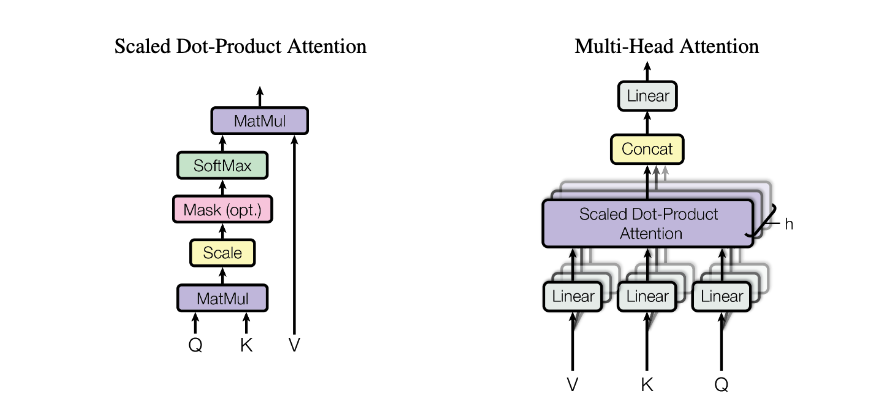
The Attention is calculated using a multi step process which takes in input as Q, K, V, and all of them are going to be the image X[t].
Essentially the left diagram above is represented as

So we simply do a matrix multiplication of Q with a transpose of K, divide it by number of channels, process it with a softmax layer and again do a matrix multiplication with V to bring it back to original dimensions.
Then to do a multi head attention, we repeat the above process multiple times and concatenate all of them, pass it through a linear layer to bring it back to original dimension.
The code for this is https://github.com/hojonathanho/diffusion/blob/master/diffusion_tf/models/unet.py Method is attn_block.

The Attention model is integrated in U-Net model only at the 16×16 feature map resolution, and uses GroupNormalization.

The Diffusion model

To train the model, we will take the input images, iterate over them one by one.

Remember to get X[t-1] from X[t] we have to use formula 1.

In the paper the authors have used the value of beta as a linear distribution between 0.0001 and 0.02 divided into T steps.
So we will have to build a list of all values of beta from beta[0] .. beta[t-1], beta [t], .. beta[T]
alphas will be 1 – betas as defined in equation 4
We can have a method to get the noisy image which will take in the X[0] the original image, the timestep where we want to generate it, and the epsilon value of the noise. And remember the Step 5 value in parentheses is the noisy image. which needs X[0], epsilon and alpha, and to get alpha we need a beta value which we are defining above.

To do the training, we have to define the training model (DiffusionModel) from keras.Model,override the train_step as follows

Get a random t (timestep) between 0 and T
Get a random epsilon noise between 0 and 1
Get the noisy image based on above logic
Pass the noisy image and t in the above model to get the epsilon-theta (the noise in the image as predicted by model)
Then we use the MeanSquaredError loss function to compare between epsilon (noise introduced) and epsilon-theta (noise predicted)
Get the partial derivatives, and do a gradient decent.

Once we have the training model, all we have to do is call the fit method on the above defined DiffusionModel with all the images in our library.

The Sampling Model

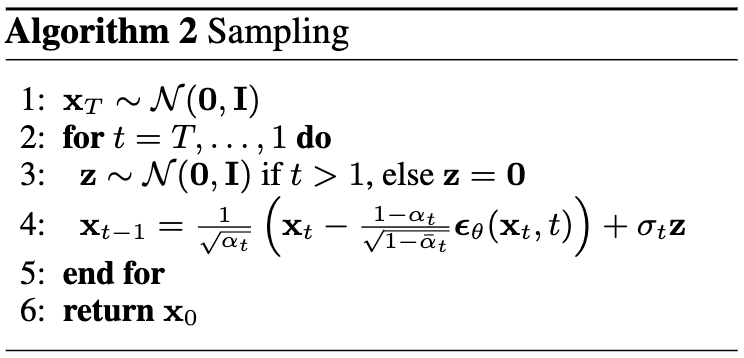
Now we generate the picture of a person from a given random noise
In Step 4, we know how to calculate alpha[t], The x[t] is the noisy image from which we are extracting the noise, the model output epsilon-theta is obtained by passing X[t] and t-current_timestep to the model, Z is a random number from Step 3
From the paper in section 3.2 Sigma is defined as

Lets say we have the T value as 1000 on which we trained the model, so when we want to generate the image from the noise, the noise will be treated as the 1000th image, and we will iterate over the above loop generating image 999, 998 and so forth upto 0 to get the final clear image.