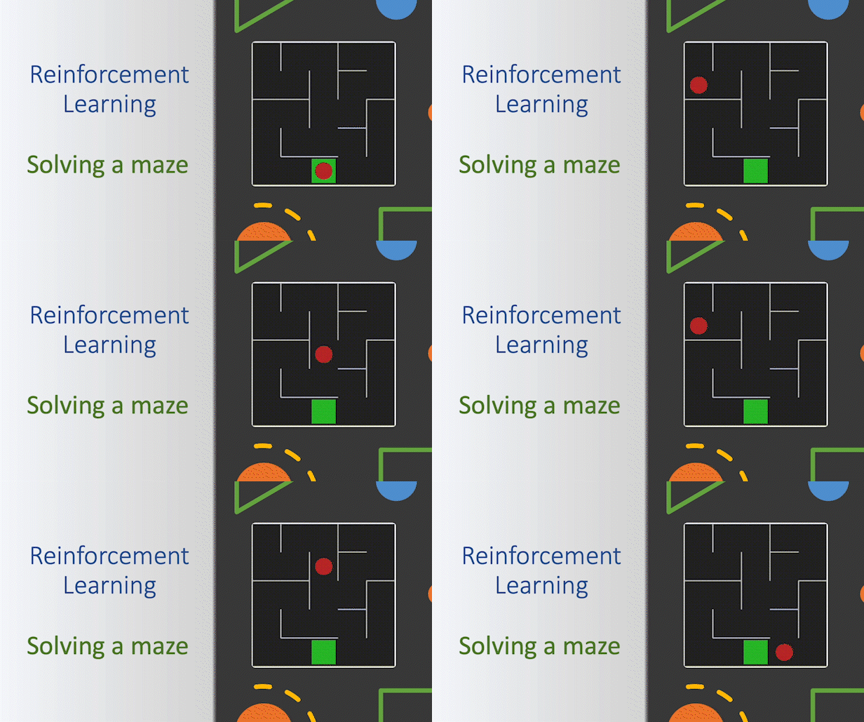
Reinforcement learning is a machine learning training method based on rewarding desired behaviors and/or punishing undesired ones. In general, a reinforcement learning agent is able to perceive and interpret its environment, take actions and learn through trial and error.
The basic concept is explained by Markov’s decision process (MDP).
There are 5 main components.
Environment: The environment is the surroundings with which the agent interacts. For example, the room where the robot moves. The agent cannot manipulate the environment; it can only control its own actions. In other words, the car can’t control where a lines are on the road, but it can act around it.
Agent: An agent is the entity which we are training to make correct decisions. For example, a ball that is being trained to move around a maze and finding an exit.
State: The state defines the current situation of the agent This can be the exact position of the ball in the maze. It all depends on how you address the problem.
Action: The choice that the agent makes at the current time step. For example, the ball can move Up, Right, Down, Left. We know defined sets of actions that the agent can perform in advance.
Policy: A policy is the thought process behind picking an action. It’s a probability distribution assigned to the set of actions. Highly rewarding actions will have a high probability and vice versa. If an action has a low probability, it doesn’t mean it won’t be picked at all. It’s just less likely to be picked.
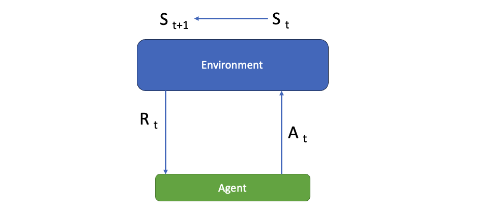
The agent takes an action which will change its state in the environment. For that action the agent will get a reward. So each action has a reward. The goal for the agent is to maximize the rewards with the policy it choses.
The Agent is in state S(0) and and it can take a action A(0) or A(1) and can land in State S(0) or S(1) depending on the action.
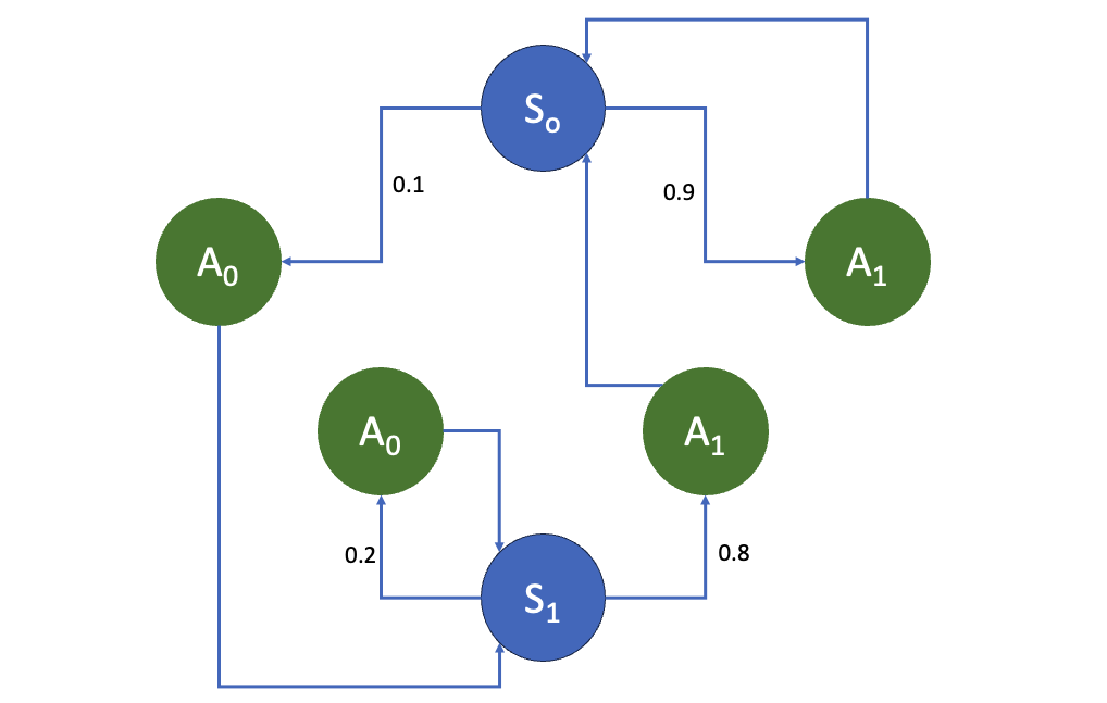
Finite: Where Actions are predined, and States are limited like a maze.
Infinite: Here we may have infinite number of states like a car on the road, where speed, location can have any value.
Moreover the MDP can be either episodic or continuous
Episodic process will terminate at some point in time (Like a game of chess)
Continuous process will never end, it simply keeps going.
Trajectory: is the trace generated when the agent moves from one state to another.

Reward: the goals of the task are represented by the rewards that the environment gives the agent in response to its actions. So in order to solve the task in the best way possible, we want to maximize the sum of those rewards. Reward is the immediate result that our actions produce.
Return: is the sum of rewards that the agent obtains from a certain point in time (t) the until the task is completed. Since we wanted to maximize the long term sum of rewards, we can also say that we want to maximize the expected return.
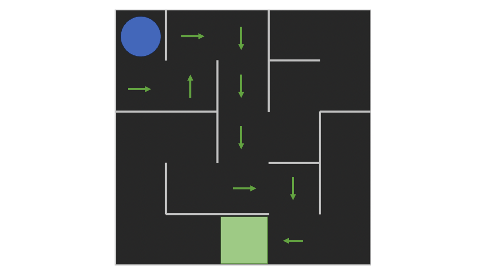
Policy: The policy is a function that takes as input a state and returns the action to be taken in that state.

import numpy as np
import matplotlib.pyplot as plt


from envs import Maze # internal code (envs)
from utils import plot_policy, plot_values, test_agent # internal code utils

env = Maze()
Display the available states and action
print(f"Observation space shape: {env.observation_space.nvec}")
print(f"Number of actions: {env.action_space.n}")

>>>Observation space shape: [5 5]
>>>>Number of actions: 4
Now create a array which will be populated later with correct probability of taking an action, right now for each state (5×5) we have 4 actions each with probability of 0.25
policy_probs = np.full((5, 5, 4), 0.25)
plot_policy(policy_probs, frame)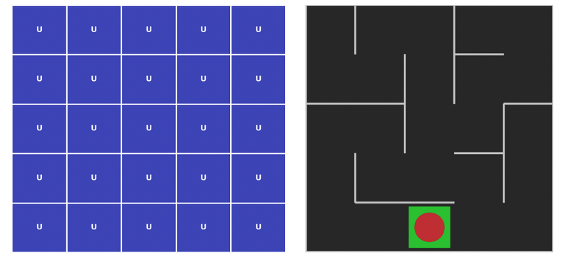
def policy(state)
   return policy_probs[state]:
Lets see how the maze is solved by random actions where probability of each action is 0.25 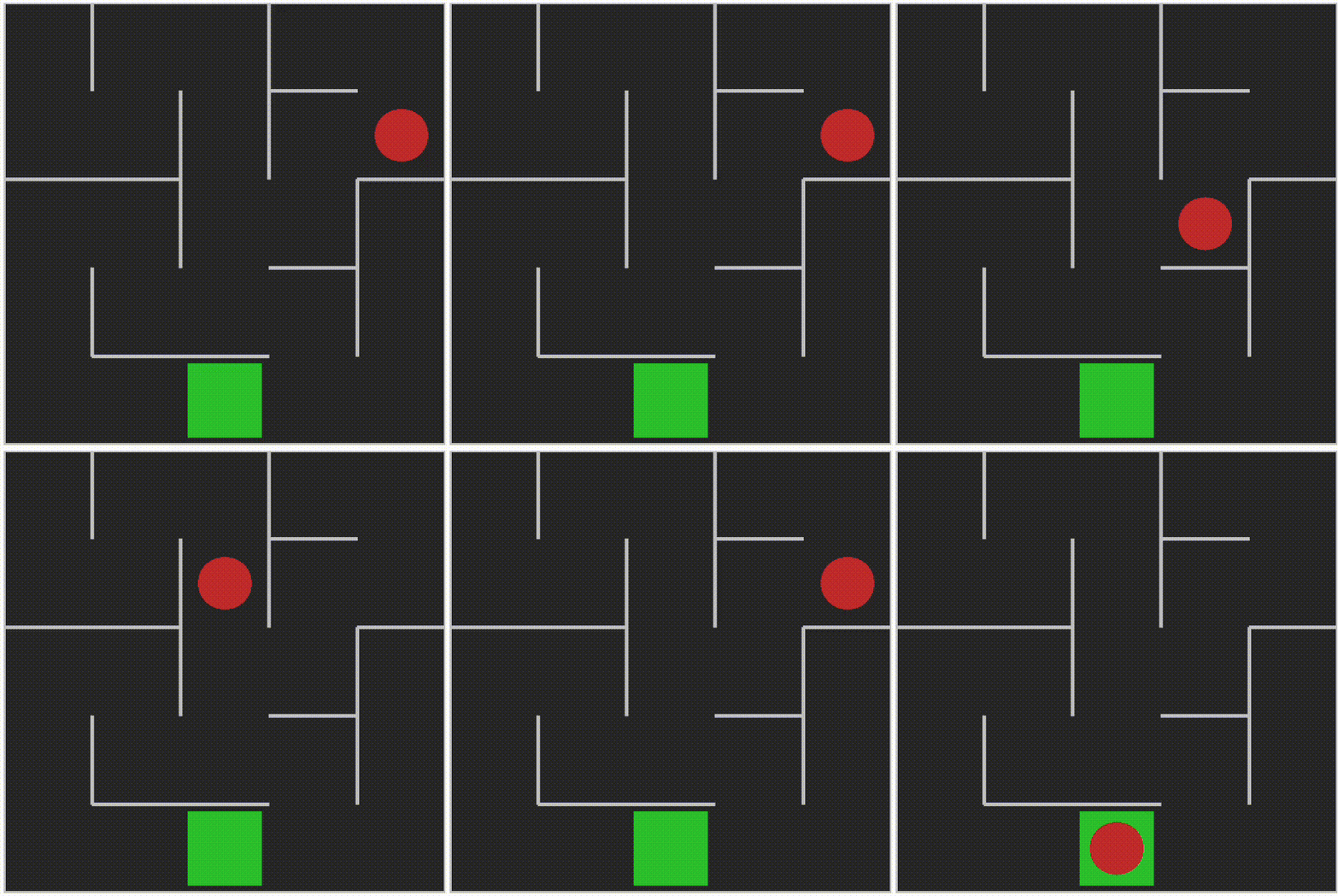
state_values = np.zeros(shape=(5,5))
plot_values(state_values, frame)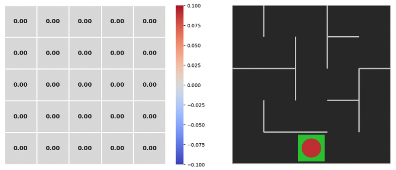
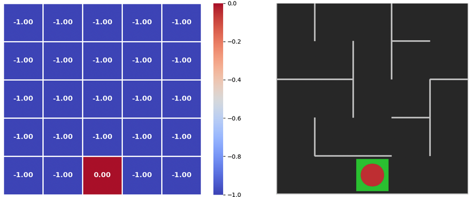
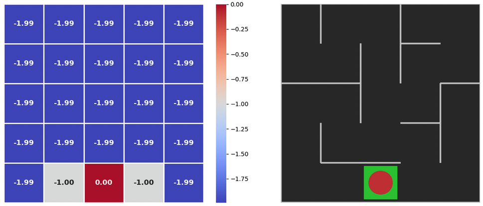
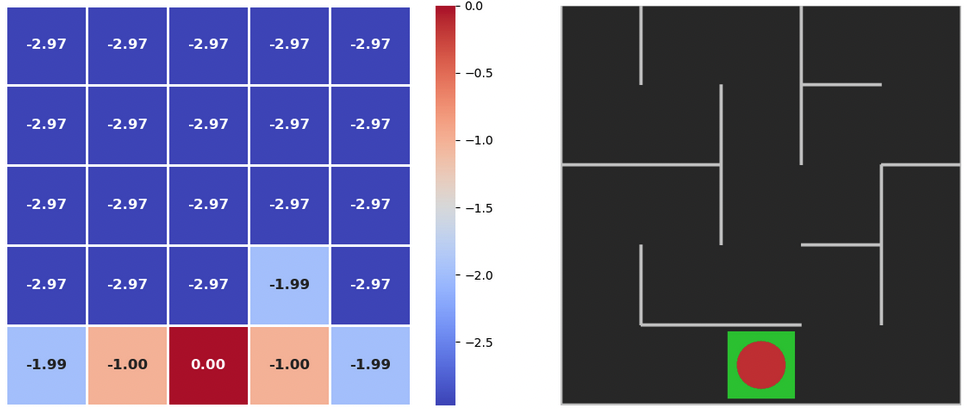
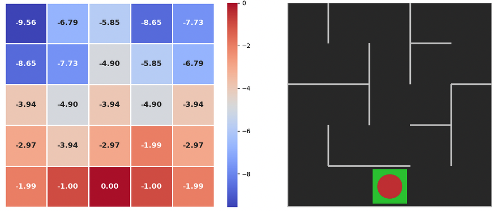
In this function, we will iterate in the maze till we see our value changes are less than a number (theta). We will reduce the reward with each step by a amount Gamma, and for each step the reward we are giving our agent is (-1) if the goal is not reached, and (0) if the goal is reached. More like a punishment than a reward.
def value_iteration(policy_probs, state_values, theta=1e-6, gamma=0.99):
    # a large value to enter the loop.
    delta = float('inf')

    while delta > theta:
        delta = 0
        plot_values(state_values, frame)
        # all the matrix
        for row in range(5):
            for col in range(5):
                old_value = state_values[(row, col)]
                # this is what we are finding
                action_probs = None
                max_qsa = float('-inf')

                # we have 4 possible actions
                for action in range(4):
                    # assume if we take the action, and move to next stage, what will be our reward
                    next_state, reward, _, _ = env.simulate_step((row, col), action)
                    # this is our return in taking the simulated action. Gamma here is the discount factor.
                    qsa = reward + gamma * state_values[next_state]
                    # find max return for the 4 actions
                    if qsa > max_qsa:
                        max_qsa = qsa
                        action_probs = np.zeros(4)
                        # assign 100% probablity to the action with max return.
                        action_probs[action] = 1.

                # update the returns
                state_values[(row, col)] = max_qsa
                # update the probablilites
                policy_probs[(row, col)] = action_probs

                # see if we can exit the loop
                delta = max(delta, abs(max_qsa - old_value))
Lets execute the function to find return values for each cell in maze
value_iteration(policy_probs, state_values)Initial values of the returns

plot_policy(policy_probs, frame)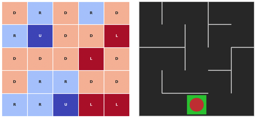
test_agent(env, policy)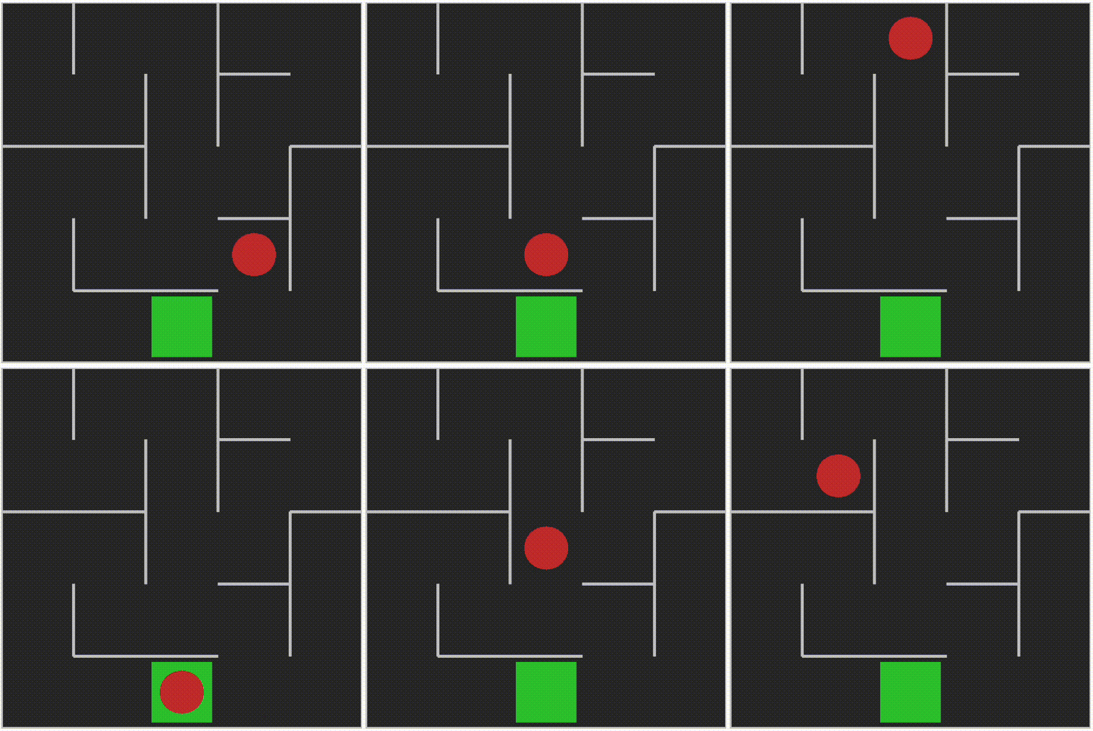
Cheers – Amit Tomar

