The attention paper we discussed in the last post created a dependency between the translated word and the original words by providing a weight to all the surrounding words, This was done to add context of the sentence to the neural network. The whole NLP, RNN enhancements are done to add this context to the word we are acting on.
In 2017 a paper was published by Google Attention is all you need, which says
We propose a new simple network architecture, the Transformer, based solely on attention mechanisms, dispensing with recurrence and convolutions entirely
What they did here, is to completely get rid of the RNN model, transferring the data from one neuron to the next within a layer and just relied on Attention and a positional matrix which provides the relevancy of other words to this word.
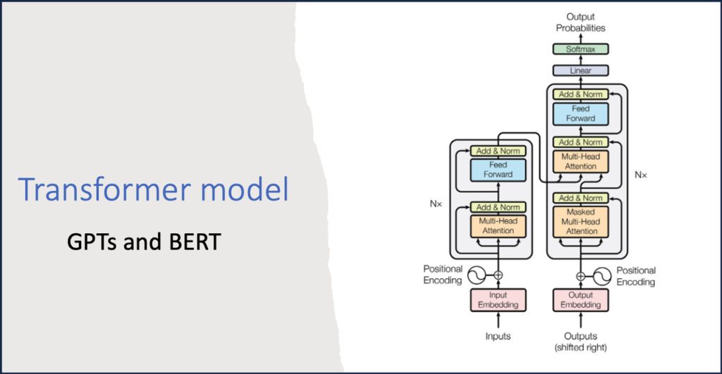
The whole transformer model looks like this.
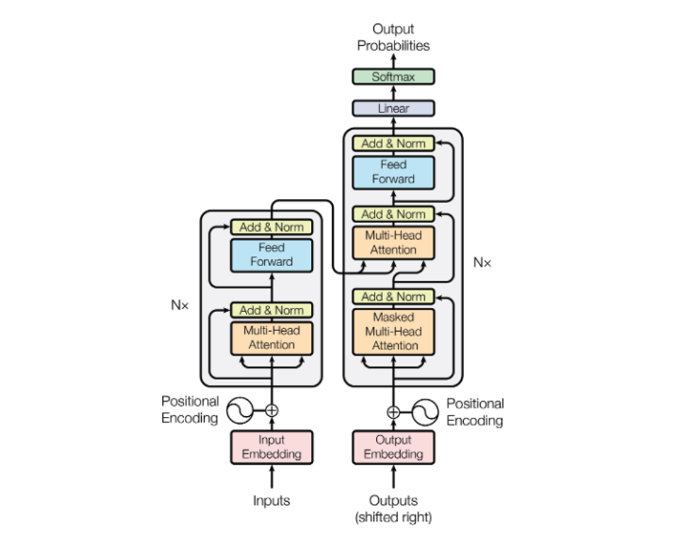
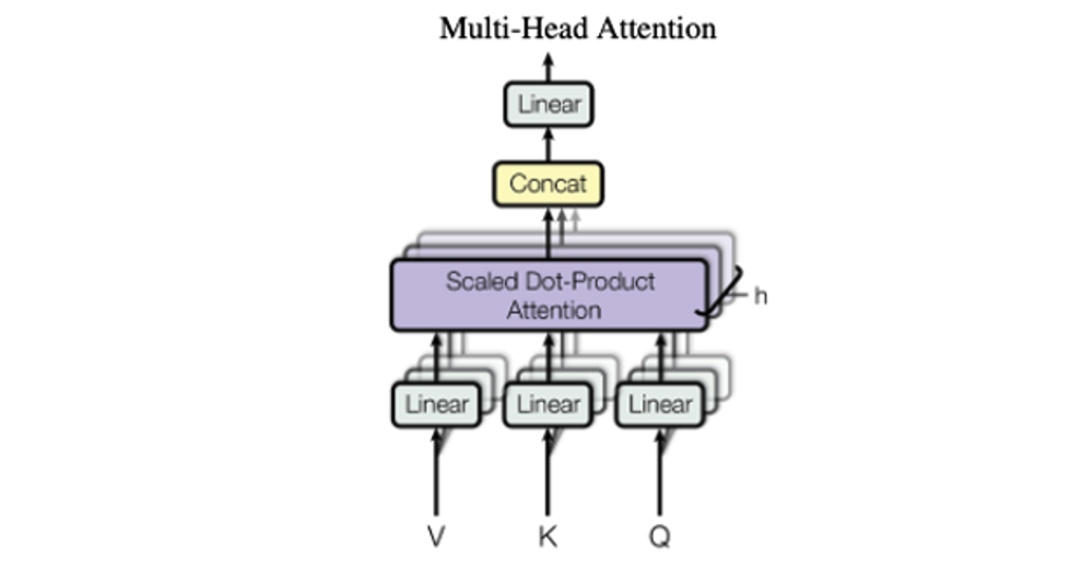
The orange boxes in it are Multi head attentions steps which are expanded to
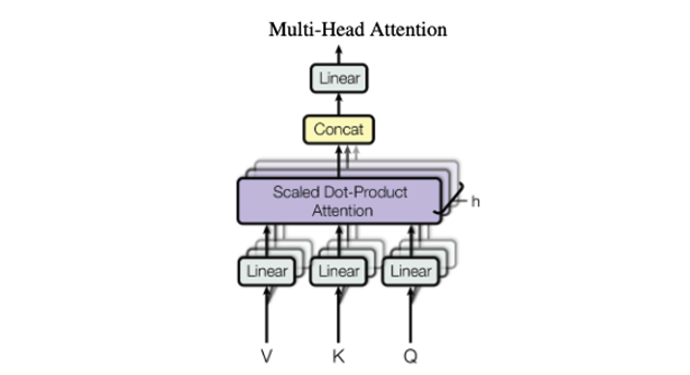
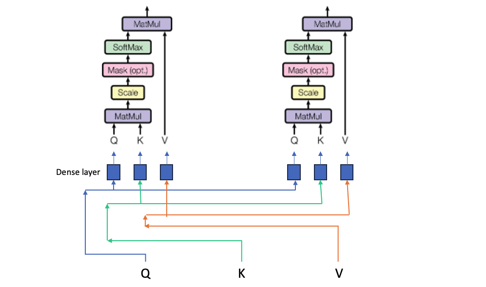
In this the purple box is the Scaled dot product attention which again gets expanded to
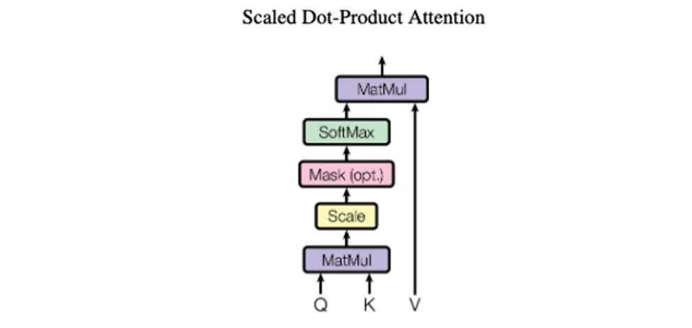
In Bahdanau’s paper, he had the original and the translated text for attention, Here since we have the original text on both dimensions, we end up having same value for Q and K above which is a matrix of sequence length X embedding dimension.
And the attention matrix after scaling looks like
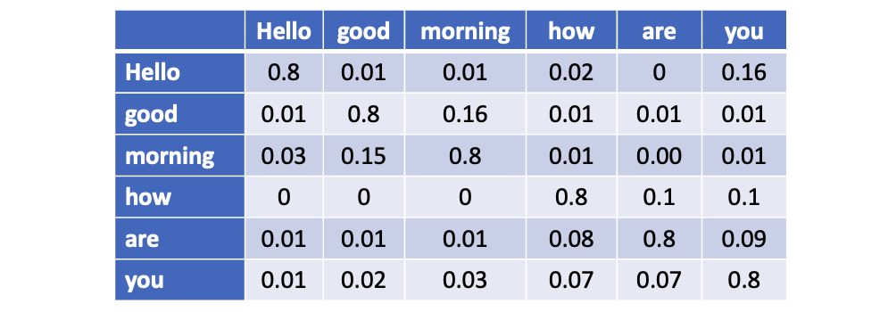
and resultant matrix is a square of dimension of sequence length. The Attention formula is defined as

The matrix above is the first part of the formula which is softmax of the Query matrix divided by root of embedding dimension.
This we multiply by the Value matrix which is the embedding matrix of the input keys, this will give us a output of same matrix dimension as the Value matrix
Before we send the data in the transformer model, we provide a positional encoding signifying which word is where in the input, and we multiply our input matrix with this to add the information about which word occurs where in the sentence.
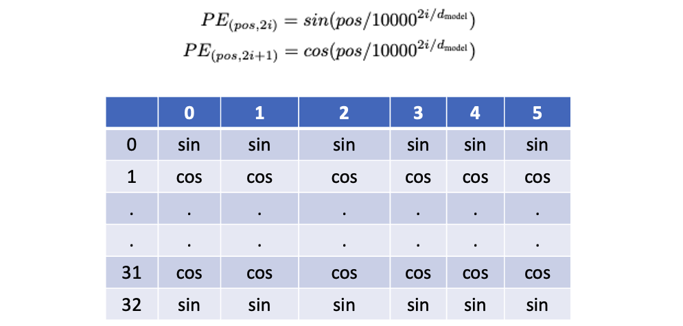
This is a static matrix for a given size, where even rows are sin, and odds are cos values. the d(model) is the dimension of our embedding matrix.
The Multi head attention model is the group of scaled dot attention models with different learned linear projections which are all then concatenated and passed through a linear layer to reduce the dimension back to the original output of a single scaled dot attention transformer.
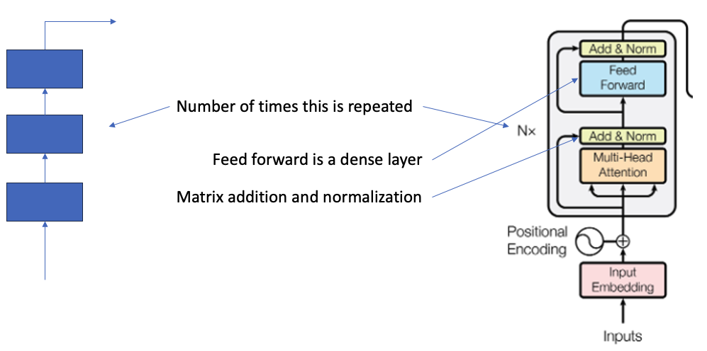
The rest of the transformation is straightforward , There is a bypass of the input which is coming to the output of the Multi head attention layer and getting Normalized again to preserve some original context. Then we have a Feed forward layer which is a simple dense layer, and we repeat this whole layer Nx times by chaining them linearly.
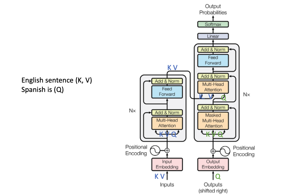
The right side of the transformer model is the decoder layer and in the Multi-head attention layer, it adds a masking layer. The mask is to prevent the model from looking ahead at the training output since it won’t be available in real life scenario. So we create a diagonal matrix which masks the future values in responses

Putting it together for a translation use-case, we pass the english sentence in the encoder and the spanish sentence goes to the decoder.
Transfer learning
As the name implies, we use the models which were trained on large number of parameters with a large dataset, and train them on a smaller task. Example we can take a model which efficiently interprets english language and then train if for sentiment analysis, or a text summarization task, or a next word prediction task.
In this mechanism we take the Model A which is already trained on large dataset, and use a smaller dataset for our task

When we are training the model on new data, we keep the learning rate low, and freeze some portions of the original model so as to keep the original knowledge preserved

GPT – Generative Pre-training Transformer model
The GPT model utilizes the decoder side of the transformer model, and gets rid of some tasks.
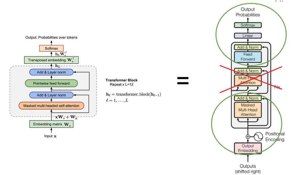
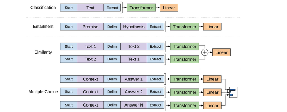
It fine tunes the same model for all end tasks. It uses Byte pair encoding to segment each word to avoid misspellings in inputs.
GPT is fine tuned on following tasks
BERT – Bidirectional Encoder Representations from Transformers
BERT utilizes the left side of the model. It is fine tuned for separate tasks in different ways
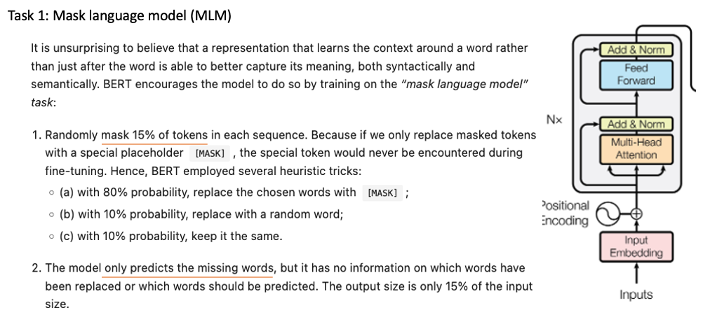
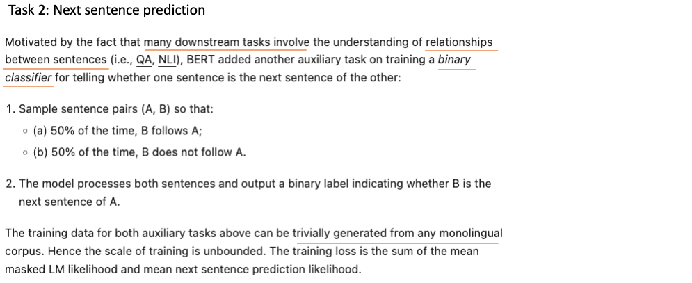
It passes an additional embedding information as a input to distinguish the 2 sentences in use cases for translations, summarization, question answers.

and uses different portions of outputs in different usecases
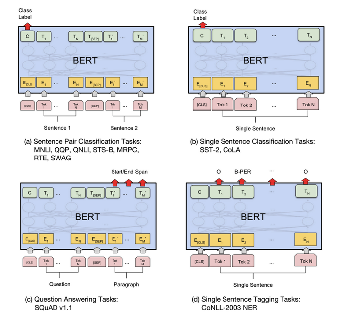
Sentence pair classification task – to check if 2 sentences mean the same thing. The output is the Class label output.
Single sentence Classification task – for this a good example is Sentiment analysis, the output here also is just the class label output which gives a positive or negative sentiment.
Question Answer task – takes in the full answer to the question and identifies the portion of the answer where the key information lies by tagging it as start and end span.
Single Sentence tagging – is a feature where we identifies and classifies words in the sentence into categories like Name, Place, job, color etc.
GPT-2
This is similar to GPT, but trained on 1.5 billion parameters which is 10 times more than GPT. It uses a technique Zero Shot transfer. This relies on formatting of input using keywords to distinguish the use-cases
Translation tasks are simply trained using sentence pairs like (English Sentence = Spanish Sentence)
Question Answer tasks are formatted similarly with pairs on questions and answers
Summarization tasks are induced by adding TL;DR; keyword after the articles in the context.
GPT-2 also enhances on the byte sequences by excluding special characters during the merging process when forming sub words. It prevents BPT from merging characters across categories so a word like “cat” will not be merged with a punctuations like “.”, “,” “!” or “?”
It also optimizes some processing between layers with following modifications
Layer normalization was moved to the input of each sub-block
An additional layer normalization was added after the final self-attention block
A modified initialization was constructed as a function of model depth
The weights of the residual layers were initially scaled by a factor of 1 /sq(N) where N is the number of residual layers
Next time we will go into Reinforcement learning and some training some simple examples
Cheers – Amit Tomar

